Graph Neural Networks and Message Passing
"Molecules are not sequences or grids — they are graphs. To understand chemistry, we must learn on graphs."
August 2026 · Giacomo Saccaggi
Why Graphs in Healthcare?
Much of healthcare data has an inherent graph structure that traditional neural networks — designed for sequences (RNNs) or grids (CNNs) — cannot naturally capture. Consider:
- Molecules: Atoms are nodes, chemical bonds are edges. A drug's efficacy depends on its molecular structure.
- Drug-drug interactions: Drugs form a network where edges represent known interactions (synergistic or adverse).
- Protein interaction networks: Proteins interact in complex webs; understanding these interactions is crucial for drug target identification.
- Knowledge graphs: Medical concepts (diseases, symptoms, treatments) connected by semantic relationships.
- Patient similarity networks: Patients as nodes, connected if they share similar conditions or treatment histories.
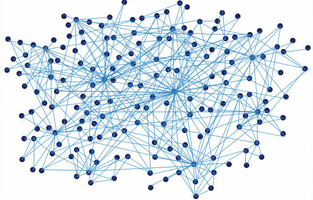
Healthcare data naturally forms graphs: molecules, drug interactions, protein networks, and knowledge graphs
Graph Learning Tasks
What can we do with graph-structured data? The tasks fall into several categories:
| Task Type | Description | Healthcare Example |
|---|---|---|
| Node Classification | Assign labels to individual nodes | Is this protein a valid drug target? Is this patient high-risk? |
| Graph Classification | Assign a label to the entire graph | Is this molecule toxic? Will this drug be effective? |
| Link Prediction | Predict missing or future edges | Will these two drugs interact adversely? |
| Graph Generation | Generate new graphs with desired properties | Design novel drug molecules with specific binding affinity |
| Node Clustering | Group similar nodes together | Identify patient subgroups with similar disease profiles |
In drug discovery, the most common task is graph-level property prediction: given a molecular graph, predict whether it will be toxic, soluble, or bind to a specific target protein.
The Node Embedding Problem
The fundamental goal of graph neural networks is to learn node embeddings — low-dimensional vector representations of nodes that capture both their features and their structural position in the graph.
Node Embedding Goal
Map each node v to a d-dimensional vector zv ∈ ℝd such that:
similarity(u, v) in network ≈ similarity(zu, zv) in embedding space
Nodes that are "similar" in the graph should have similar embeddings.
But what defines "similarity" in a graph? This is where the design choices come in:
- Connected nodes: Neighbors should be similar
- Structurally equivalent nodes: Nodes with similar local neighborhoods (even if distant)
- Nodes on same community: Belonging to the same cluster
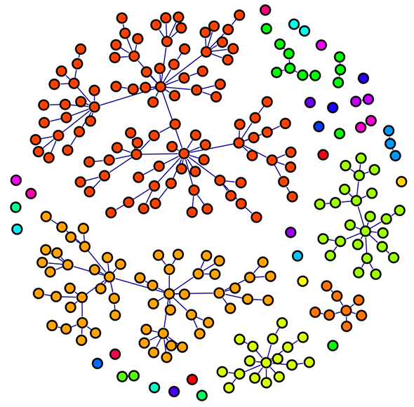
Node embeddings map graph nodes to a vector space where similar nodes are close together
Why Not Just Use Adjacency Matrix?
A naive approach would be to use the adjacency matrix row as a node's feature vector. But this has critical problems:
- High dimensionality: For a graph with N nodes, each embedding has dimension N
- Sparsity: Most entries are zeros (no edge)
- No generalization: Can't handle new nodes not seen during training
- No parameter sharing: Each node has completely independent representation
We need a function that generates embeddings based on local graph structure — this is exactly what GNNs provide.
Challenges of Learning on Graphs
Graphs are fundamentally different from the data structures deep learning was originally designed for. Here's why they're challenging:
| Challenge | Sequences/Images | Graphs |
|---|---|---|
| Size | Fixed (e.g., 224×224 image) | Arbitrary number of nodes and edges |
| Ordering | Natural order (left→right, top→bottom) | No canonical ordering of nodes |
| Locality | Local receptive fields (convolution) | No grid structure for local operations |
| Dynamics | Static once captured | Can grow/shrink over time |
| Features | Homogeneous (pixels) | Heterogeneous node and edge types |
⚠️ The Permutation Invariance Problem
If we relabel all nodes in a graph (swap node 1 with node 3, etc.), the graph is unchanged but the adjacency matrix looks completely different. Any valid graph neural network must be permutation invariant — produce the same output regardless of how nodes are numbered.
These challenges rule out directly applying CNNs or RNNs. We need architectures specifically designed for graph-structured data.
Key Ideas of Graph Neural Networks
The breakthrough insight of GNNs is elegantly simple: a node's representation should be determined by its neighborhood. Instead of learning independent embeddings, we learn how to aggregate information from neighbors.
Idea 1: Neighborhood Aggregation
Every node collects ("aggregates") information from its neighbors. If I know what my friends know, I become more informed. This is the message passing paradigm.
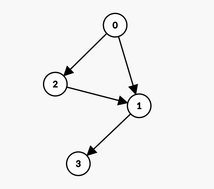
Each node aggregates information from its neighbors to update its representation
Aggregation Principle
For node v with neighbors N(v), the new representation is:
hv(new) = f(hv, AGGREGATE({hu : u ∈ N(v)}))
Where AGGREGATE is a permutation-invariant function (sum, mean, max, etc.)
The aggregation function must be permutation-invariant — the order in which we process neighbors shouldn't matter. Common choices:
- Sum: hN(v) = Σu∈N(v) hu
- Mean: hN(v) = (1/|N(v)|) × Σu∈N(v) hu
- Max: hN(v) = maxu∈N(v) hu (element-wise)
Idea 2: Multiple Layers = Larger Receptive Fields
A single aggregation step only captures immediate neighbors (1-hop). By stacking multiple layers, each node's representation incorporates information from progressively larger neighborhoods.
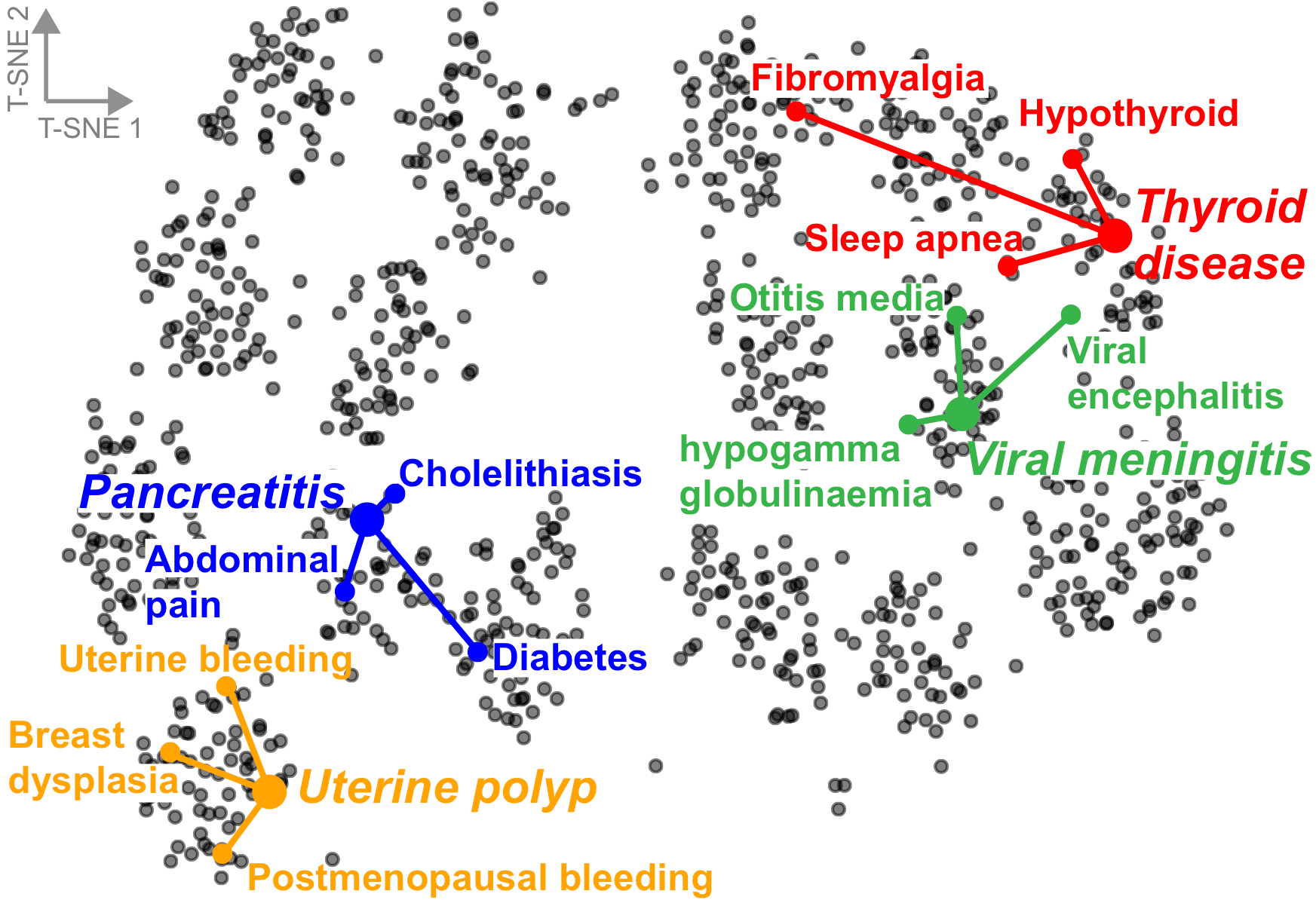
Stacking GNN layers: Layer 1 captures 1-hop neighbors, Layer 2 captures 2-hop, etc.
Layer-wise Propagation
Layer 0: hv(0) = xv (initial node features)
Layer k: hv(k) = σ(W(k) · AGGREGATE({hu(k-1) : u ∈ N(v) ∪ {v}}))
After K layers, hv(K) captures the K-hop neighborhood of node v.
This is powerful: with just 3-4 layers, most nodes in a molecular graph "see" the entire molecule. But beware of over-smoothing — with too many layers, all node embeddings converge to the same value!
💡 Receptive Field Growth
In a molecule with average degree ~3:
- 1 layer: Each atom sees ~3 neighbors
- 2 layers: Each atom sees ~9 atoms (3²)
- 3 layers: Each atom sees ~27 atoms (entire small molecule)
For drug-like molecules (20-50 atoms), 3-4 layers typically suffice.
Graph Convolutional Networks (GCN)
The Graph Convolutional Network (Kipf & Welling, 2017) is the foundational GNN architecture. It uses a simple aggregation rule inspired by spectral graph theory.
GCN Layer Definition
GCN Update Rule
For node v at layer l:
hv(l) = σ(W(l) · Σu∈N(v)∪{v} (1/√(d̃u·d̃v)) · hu(l-1))
Where:
- d̃v = degree(v) + 1 (with self-loop)
- W(l) is the learnable weight matrix for layer l
- σ is an activation function (typically ReLU)
The normalization by √(d̃u·d̃v) prevents nodes with many neighbors from having exploding activations.
Matrix Formulation
The beauty of GCN is that it can be expressed as efficient matrix operations:
GCN in Matrix Form
H(l) = σ(Â · H(l-1) · W(l))
Where:
- H(l) ∈ ℝN×d is the matrix of all node embeddings at layer l
- Â = D̃-½ · Ã · D̃-½ is the normalized adjacency matrix
- Ã = A + I (adjacency with self-loops)
- D̃ is the degree matrix of Ã
import torch import torch.nn as nn import torch.nn.functional as F class GCNLayer(nn.Module): """Single Graph Convolutional Layer.""" def __init__(self, in_features, out_features): super().__init__() self.linear = nn.Linear(in_features, out_features, bias=False) def forward(self, x, adj_normalized): """ Args: x: Node features [N, in_features] adj_normalized: Normalized adjacency matrix  [N, N] Returns: Updated node features [N, out_features] """ # Aggregate neighbor features:  · X support = torch.mm(adj_normalized, x) # Transform: ( · X) · W output = self.linear(support) return output class GCN(nn.Module): """Two-layer GCN for node classification.""" def __init__(self, n_features, n_hidden, n_classes, dropout=0.5): super().__init__() self.gcn1 = GCNLayer(n_features, n_hidden) self.gcn2 = GCNLayer(n_hidden, n_classes) self.dropout = dropout def forward(self, x, adj_normalized): # Layer 1: features → hidden h = self.gcn1(x, adj_normalized) h = F.relu(h) h = F.dropout(h, self.dropout, training=self.training) # Layer 2: hidden → output h = self.gcn2(h, adj_normalized) return h # Logits for each node
GCN Limitations
GCN is elegant but limited:
- No edge features: GCN only uses adjacency (edge exists or not). In molecules, bond type (single, double, triple, aromatic) is crucial!
- Fixed aggregation: All neighbors contribute equally (after normalization). Some neighbors may be more important.
- Scalability: Full-batch training requires the entire graph in memory.
Scalable GCN: Sampling Approaches
For large graphs, full-batch GCN is infeasible. Two popular solutions:
| Method | Idea | Trade-off |
|---|---|---|
| GraphSAGE | Sample a fixed number of neighbors per node at each layer | Variance from sampling, but constant memory per batch |
| FastGCN | Sample nodes at each layer independently using importance sampling | More efficient but can miss important connections |
# GraphSAGE-style sampling: sample k neighbors per node
def sample_neighbors(node_ids, adj_list, num_samples):
    """Sample fixed number of neighbors for each node."""
    sampled = []
    for node in node_ids:
        neighbors = adj_list[node]
        if len(neighbors) >= num_samples:
            sampled_neighbors = np.random.choice(neighbors, num_samples, replace=False)
        else:
            # Sample with replacement if not enough neighbors
            sampled_neighbors = np.random.choice(neighbors, num_samples, replace=True)
        sampled.append(sampled_neighbors)
    return np.array(sampled)
Message Passing Neural Networks (MPNN)
The Message Passing Neural Network (Gilmer et al., ICML 2017) is a general framework that unifies and extends previous GNN architectures. Crucially for drug discovery, MPNN handles both node features and edge features.
A molecule represented as a graph: atoms are nodes with features (element type, charge, hybridization), bonds are edges with features (single/double/triple, conjugated, in ring)
The MPNN Framework
MPNN operates in two phases:
- Message Passing Phase: Nodes exchange information with neighbors for T time steps
- Readout Phase: Aggregate all node embeddings into a single graph-level embedding
Message Passing Phase
At each time step t:
1. Compute messages:
mvt+1 = Σw∈N(v) Mt(hvt, hwt, evw)
2. Update node states:
hvt+1 = Ut(hvt, mvt+1)
Where:
- Mt is the message function (learnable)
- Ut is the update function (typically GRU or LSTM)
- evw is the edge feature between v and w
The key innovation is the message function Mt that incorporates edge features. In molecules, this lets the model learn that information flows differently across single vs. double bonds.
Readout Phase
After T message passing steps, aggregate node embeddings into a graph embedding:
ĥG = R({hvT | v ∈ G})
The readout function R must be permutation-invariant. Options:
- Sum pooling: ĥG = Σv hvT
- Mean pooling: ĥG = (1/|V|) × Σv hvT
- Max pooling: ĥG = maxv hvT
- Set2Set: Attention-based aggregation (more expressive)
Readout phase: all node embeddings are aggregated into a single graph-level representation
Edge-Conditioned Message Function
A common choice for Mt is the edge-conditioned convolution:
Edge Network Message Function
Mt(hv, hw, evw) = A(evw) · hw
Where A(evw) is a neural network that outputs a d×d matrix based on edge features.
This means: the edge features determine how the neighbor's information is transformed before being sent.
For efficiency, A is typically implemented as:
class EdgeNetwork(nn.Module):
    """Network that produces transformation matrix from edge features."""

    def __init__(self, edge_dim, hidden_dim):
        super().__init__()
        # Edge features → transformation matrix (flattened)
        self.net = nn.Sequential(
            nn.Linear(edge_dim, hidden_dim * 2),
            nn.ReLU(),
            nn.Linear(hidden_dim * 2, hidden_dim * hidden_dim)
        )
        self.hidden_dim = hidden_dim

    def forward(self, edge_features):
        """
        Args:
            edge_features: [num_edges, edge_dim]
        Returns:
            Transformation matrices: [num_edges, hidden_dim, hidden_dim]
        """
        flat = self.net(edge_features)  # [num_edges, hidden_dim²]
        return flat.view(-1, self.hidden_dim, self.hidden_dim)
GRU Update Function
The update function combines the node's current state with incoming messages. Using a GRU allows the model to selectively retain or forget information:
class MPNNUpdate(nn.Module):
    """GRU-based update function for MPNN."""

    def __init__(self, hidden_dim):
        super().__init__()
        self.gru = nn.GRUCell(hidden_dim, hidden_dim)

    def forward(self, h, m):
        """
        Args:
            h: Current node states [num_nodes, hidden_dim]
            m: Aggregated messages [num_nodes, hidden_dim]
        Returns:
            Updated node states [num_nodes, hidden_dim]
        """
        return self.gru(m, h)
Complete MPNN Implementation
Let's build a complete MPNN for molecular property prediction in PyTorch.
Molecular Graph Representation
First, we need to represent molecules as graphs with appropriate features:
import torch
import numpy as np
from rdkit import Chem

def atom_features(atom):
    """Extract features for a single atom."""
    return np.array([
        # Atom type (one-hot): C, N, O, S, F, Cl, Br, I, P, other
        atom.GetAtomicNum() == 6,   # Carbon
        atom.GetAtomicNum() == 7,   # Nitrogen
        atom.GetAtomicNum() == 8,   # Oxygen
        atom.GetAtomicNum() == 16,  # Sulfur
        atom.GetAtomicNum() == 9,   # Fluorine
        atom.GetAtomicNum() == 17,  # Chlorine
        atom.GetAtomicNum() == 35,  # Bromine
        atom.GetAtomicNum() == 53,  # Iodine
        atom.GetAtomicNum() == 15,  # Phosphorus
        # Degree (one-hot): 0, 1, 2, 3, 4, 5+
        atom.GetDegree() == 0,
        atom.GetDegree() == 1,
        atom.GetDegree() == 2,
        atom.GetDegree() == 3,
        atom.GetDegree() == 4,
        atom.GetDegree() >= 5,
        # Formal charge
        atom.GetFormalCharge(),
        # Num hydrogens
        atom.GetTotalNumHs(),
        # Aromaticity
        atom.GetIsAromatic(),
        # In ring
        atom.IsInRing(),
    ], dtype=np.float32)


def bond_features(bond):
    """Extract features for a single bond."""
    bt = bond.GetBondType()
    return np.array([
        # Bond type (one-hot)
        bt == Chem.rdchem.BondType.SINGLE,
        bt == Chem.rdchem.BondType.DOUBLE,
        bt == Chem.rdchem.BondType.TRIPLE,
        bt == Chem.rdchem.BondType.AROMATIC,
        # Conjugation
        bond.GetIsConjugated(),
        # In ring
        bond.IsInRing(),
    ], dtype=np.float32)


def mol_to_graph(smiles):
    """Convert SMILES string to graph representation."""
    mol = Chem.MolFromSmiles(smiles)
    if mol is None:
        return None

    # Node features
    atom_feats = np.array([atom_features(atom) for atom in mol.GetAtoms()])

    # Edge indices and features
    edge_indices = []
    edge_feats = []
    for bond in mol.GetBonds():
        i, j = bond.GetBeginAtomIdx(), bond.GetEndAtomIdx()
        bf = bond_features(bond)
        # Add both directions (undirected graph)
        edge_indices.append([i, j])
        edge_indices.append([j, i])
        edge_feats.append(bf)
        edge_feats.append(bf)

    edge_index = np.array(edge_indices).T  # [2, num_edges]
    edge_attr = np.array(edge_feats)        # [num_edges, edge_dim]

    return {
        'node_features': atom_feats,
        'edge_index': edge_index,
        'edge_features': edge_attr,
        'num_nodes': len(atom_feats)
    }
The MPNN Model
import torch
import torch.nn as nn

class MPNN(nn.Module):
    """Message Passing Neural Network for molecular property prediction."""

    def __init__(self, node_dim, edge_dim, hidden_dim, output_dim,
                 num_message_passing=3, dropout=0.1):
        super().__init__()

        self.hidden_dim = hidden_dim
        self.num_message_passing = num_message_passing

        # Initial node embedding
        self.node_encoder = nn.Linear(node_dim, hidden_dim)

        # Edge network: edge features → transformation matrix
        self.edge_network = nn.Sequential(
            nn.Linear(edge_dim, hidden_dim),
            nn.ReLU(),
            nn.Linear(hidden_dim, hidden_dim * hidden_dim)
        )

        # GRU for node state updates
        self.gru = nn.GRUCell(hidden_dim, hidden_dim)

        # Readout network
        self.readout = nn.Sequential(
            nn.Linear(hidden_dim, hidden_dim),
            nn.ReLU(),
            nn.Dropout(dropout),
            nn.Linear(hidden_dim, output_dim)
        )

    def forward(self, node_features, edge_index, edge_features, batch):
        """
        Args:
            node_features: [total_nodes, node_dim] - all nodes in batch
            edge_index: [2, total_edges] - edge connectivity
            edge_features: [total_edges, edge_dim] - edge attributes
            batch: [total_nodes] - graph membership for each node
        Returns:
            Graph-level predictions: [batch_size, output_dim]
        """
        # Initial node embeddings
        h = self.node_encoder(node_features)  # [N, hidden_dim]

        # Compute edge transformations once
        edge_transform = self.edge_network(edge_features)  # [E, hidden_dim²]
        edge_transform = edge_transform.view(-1, self.hidden_dim, self.hidden_dim)

        # Message passing iterations
        for _ in range(self.num_message_passing):
            h = self.message_passing_step(h, edge_index, edge_transform)

        # Readout: aggregate node embeddings per graph
        graph_embed = self.global_mean_pool(h, batch)  # [batch_size, hidden_dim]

        # Final prediction
        out = self.readout(graph_embed)
        return out

    def message_passing_step(self, h, edge_index, edge_transform):
        """Single message passing step."""
        source, target = edge_index  # [E], [E]

        # Get source node embeddings
        h_source = h[source]  # [E, hidden_dim]

        # Apply edge-conditioned transformation: A(e) @ h_source
        # edge_transform: [E, hidden_dim, hidden_dim]
        # h_source: [E, hidden_dim] → [E, hidden_dim, 1]
        messages = torch.bmm(edge_transform, h_source.unsqueeze(-1)).squeeze(-1)

        # Aggregate messages per target node
        num_nodes = h.size(0)
        aggregated = torch.zeros(num_nodes, self.hidden_dim, device=h.device)
        aggregated.scatter_add_(0, target.unsqueeze(-1).expand_as(messages), messages)

        # Update node states with GRU
        h_new = self.gru(aggregated, h)
        return h_new

    def global_mean_pool(self, h, batch):
        """Average pooling over nodes in each graph."""
        batch_size = batch.max().item() + 1

        # Sum node embeddings per graph
        graph_sum = torch.zeros(batch_size, h.size(1), device=h.device)
        graph_sum.scatter_add_(0, batch.unsqueeze(-1).expand_as(h), h)

        # Count nodes per graph
        ones = torch.ones(h.size(0), device=h.device)
        count = torch.zeros(batch_size, device=h.device)
        count.scatter_add_(0, batch, ones)

        # Mean
        graph_embed = graph_sum / count.unsqueeze(-1).clamp(min=1)
        return graph_embed
Training Loop
def train_mpnn(model, train_loader, val_loader, epochs=100, lr=0.001):
    """Train MPNN for molecular property prediction."""
    device = torch.device('cuda' if torch.cuda.is_available() else 'cpu')
    model = model.to(device)

    optimizer = torch.optim.Adam(model.parameters(), lr=lr)
    criterion = nn.MSELoss()  # For regression; use BCEWithLogitsLoss for classification

    best_val_loss = float('inf')

    for epoch in range(epochs):
        # Training
        model.train()
        train_loss = 0
        for batch in train_loader:
            batch = batch.to(device)

            optimizer.zero_grad()
            pred = model(batch.x, batch.edge_index, batch.edge_attr, batch.batch)
            loss = criterion(pred.squeeze(), batch.y)
            loss.backward()
            optimizer.step()

            train_loss += loss.item() * batch.num_graphs

        train_loss /= len(train_loader.dataset)

        # Validation
        model.eval()
        val_loss = 0
        with torch.no_grad():
            for batch in val_loader:
                batch = batch.to(device)
                pred = model(batch.x, batch.edge_index, batch.edge_attr, batch.batch)
                loss = criterion(pred.squeeze(), batch.y)
                val_loss += loss.item() * batch.num_graphs

        val_loss /= len(val_loader.dataset)

        if val_loss < best_val_loss:
            best_val_loss = val_loss
            torch.save(model.state_dict(), 'best_mpnn.pt')

        if (epoch + 1) % 10 == 0:
            print(f'Epoch {epoch+1:3d} | Train Loss: {train_loss:.4f} | Val Loss: {val_loss:.4f}')

    return best_val_loss
💡 MPNN vs GCN: When to Use What
Use GCN when:
- Edge features are not important (social networks, citation graphs)
- You need fast training on large graphs
- Task is node classification or link prediction
Use MPNN when:
- Edge features are crucial (molecules: bond types matter!)
- Task is graph-level property prediction
- Graphs are relatively small (< 100 nodes typical for molecules)
Graph Attention Networks (GAT)
Standard GCN treats all neighbors equally (after degree normalization). But in many applications, some neighbors are more important than others. Graph Attention Networks (Veličković et al., ICLR 2018) learn to weight neighbors differently using attention.
Attention Mechanism
For each edge (i, j), compute an attention coefficient:
GAT Attention
Step 1: Compute raw attention scores:
eij = LeakyReLU(aT · [W·hi || W·hj])
Step 2: Normalize using softmax over neighbors:
αij = softmaxj(eij) = exp(eij) / Σk∈N(i) exp(eik)
Step 3: Weighted aggregation:
hi' = σ(Σj∈N(i) αij · W · hj)
Where:
- W is a learnable weight matrix
- a is a learnable attention vector
- || denotes concatenation

GAT computes attention weights for each neighbor, allowing the model to focus on the most relevant connections
Multi-head Attention
Like Transformers, GAT benefits from multiple attention heads that learn different aspects of neighbor importance:
class GATLayer(nn.Module):
    """Graph Attention Layer with multi-head attention."""

    def __init__(self, in_dim, out_dim, num_heads=4, dropout=0.1, concat=True):
        super().__init__()
        self.num_heads = num_heads
        self.out_dim = out_dim
        self.concat = concat

        # Separate weight matrices per head
        self.W = nn.Linear(in_dim, out_dim * num_heads, bias=False)

        # Attention mechanism per head
        self.attention = nn.Parameter(torch.zeros(num_heads, 2 * out_dim))
        nn.init.xavier_uniform_(self.attention)

        self.leaky_relu = nn.LeakyReLU(0.2)
        self.dropout = nn.Dropout(dropout)

    def forward(self, h, edge_index):
        """
        Args:
            h: Node features [N, in_dim]
            edge_index: [2, E]
        Returns:
            Updated features [N, out_dim * num_heads] if concat else [N, out_dim]
        """
        N = h.size(0)

        # Linear transformation: [N, out_dim * num_heads]
        Wh = self.W(h).view(N, self.num_heads, self.out_dim)  # [N, H, D]

        source, target = edge_index

        # Get source and target node embeddings for each edge
        Wh_source = Wh[source]  # [E, H, D]
        Wh_target = Wh[target]  # [E, H, D]

        # Concatenate and compute attention scores
        edge_features = torch.cat([Wh_source, Wh_target], dim=-1)  # [E, H, 2D]
        e = (edge_features * self.attention).sum(dim=-1)  # [E, H]
        e = self.leaky_relu(e)

        # Softmax over incoming edges per node
        alpha = self.edge_softmax(e, target, N)  # [E, H]
        alpha = self.dropout(alpha)

        # Weighted aggregation
        weighted = Wh_source * alpha.unsqueeze(-1)  # [E, H, D]

        out = torch.zeros(N, self.num_heads, self.out_dim, device=h.device)
        out.scatter_add_(0, target.view(-1, 1, 1).expand_as(weighted), weighted)

        if self.concat:
            return out.view(N, -1)  # [N, H*D]
        else:
            return out.mean(dim=1)   # [N, D] - average over heads

    def edge_softmax(self, e, target, num_nodes):
        """Compute softmax over incoming edges for each node."""
        # Subtract max for numerical stability
        e_max = torch.zeros(num_nodes, e.size(1), device=e.device)
        e_max.scatter_reduce_(0, target.unsqueeze(-1).expand_as(e), e, 'amax')
        e = e - e_max[target]

        # Exp and sum
        exp_e = e.exp()
        sum_exp = torch.zeros(num_nodes, e.size(1), device=e.device)
        sum_exp.scatter_add_(0, target.unsqueeze(-1).expand_as(exp_e), exp_e)

        return exp_e / (sum_exp[target] + 1e-10)
When to Use GAT
| Scenario | GCN | GAT |
|---|---|---|
| All neighbors equally important | ✓ | Works but overkill |
| Some neighbors more relevant | Can't learn this | ✓ Learns attention weights |
| Need interpretability | Limited | ✓ Attention weights reveal importance |
| Computational budget | Faster | More parameters, slower |
MPNN for Quantum Chemistry
The original MPNN paper demonstrated state-of-the-art results on the QM9 dataset — predicting quantum mechanical properties of molecules.
QM9 Dataset
QM9 contains ~134,000 small organic molecules with up to 9 heavy atoms (C, N, O, F). For each molecule, 13 quantum chemical properties were computed using density functional theory (DFT):
| Property | Symbol | Unit | Description |
|---|---|---|---|
| Dipole moment | μ | Debye | Measure of charge separation |
| Polarizability | α | Bohr³ | Response to electric field |
| HOMO energy | εHOMO | eV | Highest occupied molecular orbital |
| LUMO energy | εLUMO | eV | Lowest unoccupied molecular orbital |
| Gap | Δε | eV | LUMO - HOMO energy |
| Zero-point energy | ZPVE | eV | Vibrational ground state energy |
| Heat capacity | Cv | cal/mol·K | At 298K |
| Atomization energy | U0 | eV | At 0K |
Results
MPNN achieved significant improvements over previous methods:
| Property | Previous Best | MPNN | Improvement |
|---|---|---|---|
| μ (Dipole) | 0.028 | 0.016 | 43% |
| α (Polar.) | 0.25 | 0.092 | 63% |
| εHOMO | 0.0036 | 0.0022 | 39% |
| Gap | 0.0047 | 0.0032 | 32% |
| ZPVE | 0.0006 | 0.00017 | 72% |
| U0 | 0.45 | 0.19 | 58% |
The HOMO-LUMO gap is particularly important in drug discovery — it correlates with molecular stability and reactivity.
Practical Considerations
Batching Graphs
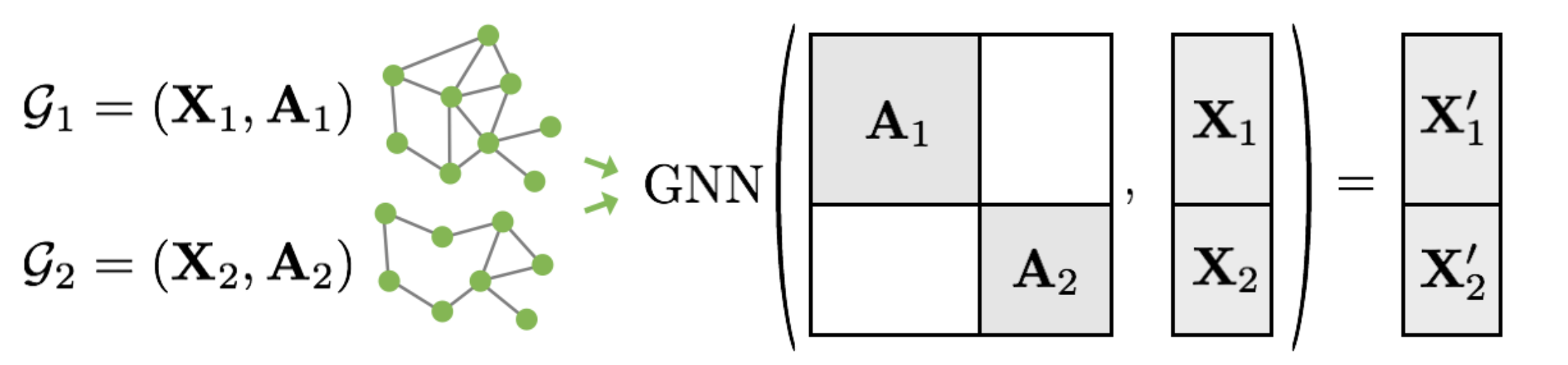
Unlike images where batching is straightforward (stack along a new dimension), graphs have variable sizes. The solution: create one large disconnected graph containing all molecules in the batch.
def collate_graphs(graphs):
    """Combine multiple graphs into a batch."""
    batch_node_features = []
    batch_edge_index = []
    batch_edge_features = []
    batch_labels = []
    batch_membership = []  # Which graph each node belongs to

    node_offset = 0
    for i, g in enumerate(graphs):
        num_nodes = g['node_features'].shape[0]

        batch_node_features.append(g['node_features'])
        batch_edge_features.append(g['edge_features'])

        # Offset edge indices
        edge_index = g['edge_index'] + node_offset
        batch_edge_index.append(edge_index)

        # Track which graph each node belongs to
        batch_membership.extend([i] * num_nodes)

        batch_labels.append(g['label'])
        node_offset += num_nodes

    return {
        'node_features': torch.cat([torch.tensor(x) for x in batch_node_features]),
        'edge_index': torch.cat([torch.tensor(x) for x in batch_edge_index], dim=1),
        'edge_features': torch.cat([torch.tensor(x) for x in batch_edge_features]),
        'batch': torch.tensor(batch_membership),
        'labels': torch.tensor(batch_labels)
    }
PyTorch Geometric
In practice, use PyTorch Geometric (PyG), which provides optimized implementations of common GNN operations:
from torch_geometric.nn import GCNConv, GATConv, NNConv, Set2Set
from torch_geometric.data import Data, DataLoader

class MPNN_PyG(nn.Module):
    """MPNN using PyTorch Geometric's NNConv (edge network convolution)."""

    def __init__(self, node_dim, edge_dim, hidden_dim, output_dim, num_layers=3):
        super().__init__()

        self.node_encoder = nn.Linear(node_dim, hidden_dim)

        # Edge network for NNConv
        edge_nn = nn.Sequential(
            nn.Linear(edge_dim, hidden_dim),
            nn.ReLU(),
            nn.Linear(hidden_dim, hidden_dim * hidden_dim)
        )

        # Message passing layers
        self.convs = nn.ModuleList()
        self.grus = nn.ModuleList()
        for _ in range(num_layers):
            self.convs.append(NNConv(hidden_dim, hidden_dim, edge_nn, aggr='add'))
            self.grus.append(nn.GRUCell(hidden_dim, hidden_dim))

        # Set2Set readout for better aggregation
        self.readout = Set2Set(hidden_dim, processing_steps=3)

        # Final MLP
        self.mlp = nn.Sequential(
            nn.Linear(2 * hidden_dim, hidden_dim),
            nn.ReLU(),
            nn.Linear(hidden_dim, output_dim)
        )

    def forward(self, data):
        x = self.node_encoder(data.x)

        for conv, gru in zip(self.convs, self.grus):
            m = conv(x, data.edge_index, data.edge_attr)
            x = gru(m, x)

        # Graph-level readout
        graph_embed = self.readout(x, data.batch)

        return self.mlp(graph_embed)
Computational Complexity
⚠️ MPNN Limitations
- Memory: O(N × d + E × d²) where N = nodes, E = edges, d = hidden dimension
- Best for small graphs: Works great for molecules (10-50 atoms) but struggles with graphs of 10,000+ nodes
- Edge network bottleneck: Computing d×d matrices per edge is expensive
For large-scale graphs (social networks, citation graphs), use GCN with sampling or more efficient architectures like GraphSAINT or ClusterGCN.
Summary
We've covered the theory and implementation of Graph Neural Networks for drug discovery:
| Architecture | Key Feature | Best For |
|---|---|---|
| GCN | Simple neighborhood aggregation | Large graphs, node classification |
| GraphSAGE | Sampling for scalability | Very large graphs, inductive learning |
| MPNN | Edge features via message functions | Molecules, small graphs with rich edge info |
| GAT | Learned attention weights | When neighbor importance varies |
Key Takeaways
- Graphs are everywhere in healthcare: molecules, drug interactions, protein networks, knowledge graphs
- GNNs learn node embeddings by aggregating information from neighbors
- Multiple layers capture larger neighborhoods: k layers = k-hop receptive field
- Edge features matter for molecules: MPNN explicitly models bond types
- Readout functions aggregate nodes into graph-level representations for property prediction
📚 Key Papers
- Kipf & Welling (2017). "Semi-Supervised Classification with Graph Convolutional Networks" — GCN
- Hamilton et al. (2017). "Inductive Representation Learning on Large Graphs" — GraphSAGE
- Gilmer et al. (2017). "Neural Message Passing for Quantum Chemistry" — MPNN
- Veličković et al. (2018). "Graph Attention Networks" — GAT
References
- Gilmer, J., Schoenholz, S.S., Riley, P.F., Vinyals, O., & Dahl, G.E. (2017). "Neural Message Passing for Quantum Chemistry". ICML 2017.
- Kipf, T.N. & Welling, M. (2017). "Semi-Supervised Classification with Graph Convolutional Networks". ICLR 2017.
- Veličković, P., Cucurull, G., Casanova, A., Romero, A., Liò, P., & Bengio, Y. (2018). "Graph Attention Networks". ICLR 2018.
- Hamilton, W.L., Ying, R., & Leskovec, J. (2017). "Inductive Representation Learning on Large Graphs". NeurIPS 2017.
- Duvenaud, D., et al. (2015). "Convolutional Networks on Graphs for Learning Molecular Fingerprints". NeurIPS 2015.
- Ramakrishnan, R., et al. (2014). "Quantum chemistry structures and properties of 134 kilo molecules". Scientific Data.