Generative Models: VAEs and GANs for Healthcare
"The goal is not to generate any data, but to generate data that is indistinguishable from real patient records while revealing nothing about actual patients."
August 2026 · Giacomo Saccaggi
Why Generate Healthcare Data?
Healthcare data is among the most sensitive and valuable resources in machine learning. Electronic Health Records (EHRs) contain detailed information about diagnoses, treatments, lab results, and outcomes — exactly what we need to train predictive models. But there's a fundamental tension:
- Privacy constraints: HIPAA, GDPR, and institutional policies restrict data sharing
- Data scarcity: Rare diseases have few examples; new hospitals have limited history
- Class imbalance: Adverse events (mortality, readmission) are rare but important
- Research reproducibility: Researchers can't share patient data, hindering replication
Generative models offer a solution: learn the underlying distribution of real patient data, then generate synthetic records that preserve statistical properties without exposing any individual patient.

Generative models learn to produce new samples from the data distribution
Generative vs Discriminative Models
Before diving into specific architectures, let's understand the fundamental distinction between two paradigms in machine learning:
| Aspect | Discriminative Models | Generative Models |
|---|---|---|
| Goal | Learn decision boundary | Learn data distribution |
| Models | P(y|x) — label given features | P(x) or P(x,y) — joint distribution |
| Examples | Logistic regression, SVM, DNNs | GANs, VAEs, Normalizing Flows |
| Output | Class labels, predictions | New samples from learned distribution |
| Use case | Classification, regression | Data augmentation, synthesis, imputation |
The Core Difference
Discriminative: Given a patient's features x, what is the probability of mortality?
P(mortality = 1 | diagnoses, labs, vitals)
Generative: What does a typical diabetic patient with heart failure look like?
P(diagnoses, labs, vitals | diabetes ∧ heart_failure)
Generative models are strictly more powerful — if you can model P(x,y), you can derive P(y|x) via Bayes' rule. But this power comes with complexity: modeling high-dimensional distributions is fundamentally harder than learning decision boundaries.
Generative Adversarial Networks (GANs)
GANs, introduced by Goodfellow et al. in 2014, represent one of the most influential ideas in deep learning. The core insight is brilliant: instead of explicitly modeling the data distribution, pit two neural networks against each other in a game.

GAN architecture: Generator creates fake samples, Discriminator distinguishes real from fake
The Two Players
Generator G: Takes random noise z ~ P(z) and transforms it into fake samples G(z) that should look like real data. Think of it as a counterfeiter trying to produce convincing fake currency.
Discriminator D: Takes a sample (real or generated) and outputs the probability that it came from the real data distribution. Think of it as a detective trying to catch counterfeits.
The Minimax Game
The two networks play a minimax game with the following objective:
GAN Objective Function
minG maxD V(D, G) = 𝔼x~pdata[log D(x)] + 𝔼z~pz[log(1 - D(G(z)))]
Discriminator's goal: Maximize V — correctly classify real samples as real (D(x)→1) and fake samples as fake (D(G(z))→0)
Generator's goal: Minimize V — fool the discriminator so D(G(z))→1
Training Procedure
Training alternates between updating D and G:
# GAN Training Algorithm (simplified)
for epoch in range(num_epochs):
    for real_batch in dataloader:

        # ============ Train Discriminator ============
        # Goal: maximize log D(x) + log(1 - D(G(z)))

        # Sample random noise
        z = torch.randn(batch_size, latent_dim)

        # Generate fake samples
        fake_batch = G(z).detach()  # detach to avoid backprop through G

        # Discriminator predictions
        real_pred = D(real_batch)
        fake_pred = D(fake_batch)

        # Discriminator loss: maximize log D(real) + log(1 - D(fake))
        # Equivalent to minimize -log D(real) - log(1 - D(fake))
        d_loss = -torch.mean(torch.log(real_pred)) - torch.mean(torch.log(1 - fake_pred))

        d_optimizer.zero_grad()
        d_loss.backward()
        d_optimizer.step()

        # ============ Train Generator ============
        # Goal: minimize log(1 - D(G(z))) ≈ maximize log D(G(z))

        z = torch.randn(batch_size, latent_dim)
        fake_batch = G(z)
        fake_pred = D(fake_batch)

        # Generator loss: maximize log D(G(z))
        # In practice, minimize -log D(G(z)) for better gradients
        g_loss = -torch.mean(torch.log(fake_pred))

        g_optimizer.zero_grad()
        g_loss.backward()
        g_optimizer.step()
⚠️ Training Instability
GAN training is notoriously unstable. Common issues:
- Mode collapse: Generator produces limited variety of samples
- Vanishing gradients: If D becomes too good, G gets no useful gradient signal
- Oscillation: D and G alternate between winning, never converging
Convergence is an open problem — there's no guarantee GANs reach equilibrium!
The Generator Loss Trick
In the original formulation, G minimizes log(1 - D(G(z))). But when D is confident (D(G(z)) ≈ 0), this gradient vanishes. In practice, we use:
Practical Generator Loss
Original: minG log(1 - D(G(z))) — saturates when D is good
Practical: maxG log D(G(z)) — stronger gradients early in training
Both have the same fixed point, but the practical version has better gradient flow.
MedGAN: Generating Synthetic EHR Data
Standard GANs work well for continuous data like images, but EHR data is fundamentally different: it's discrete (binary diagnosis codes), multi-label (patients have multiple conditions), and high-dimensional (thousands of possible codes).
MedGAN (Choi et al., 2017) addresses these challenges by combining an autoencoder with a GAN, operating in a continuous latent space rather than directly on discrete codes.

MedGAN architecture: Autoencoder + GAN for discrete EHR generation
The Discrete Data Problem
Why can't we use a standard GAN for binary medical codes?
- Non-differentiable: Binary outputs break gradient flow
- Sparse: Most patients have very few codes out of thousands
- Structured: Codes have semantic relationships (ICD hierarchy)
MedGAN Architecture
MedGAN uses a two-stage approach:
| Component | Input | Output | Purpose |
|---|---|---|---|
| Encoder (Enc) | Binary codes x | Continuous h | Map discrete to continuous |
| Decoder (Dec) | Continuous h | Binary codes x̂ | Map continuous to discrete |
| Generator (G) | Noise z | Continuous h' | Generate in latent space |
| Discriminator (D) | Binary codes | Real/Fake prob | Distinguish real from fake |
Training Procedure
Stage 1: Pre-train Autoencoder
Train Enc/Dec to reconstruct real patient records:
Autoencoder Loss
LAE = ||x - Dec(Enc(x))||²
This creates a smooth latent space where similar patients map to nearby points.
Stage 2: Train GAN in Latent Space
Generator produces latent codes, Decoder maps to discrete, Discriminator judges:
# MedGAN Training (Stage 2)
for epoch in range(num_epochs):
    for real_x in dataloader:

        # ============ Train Discriminator ============
        z = torch.randn(batch_size, noise_dim)

        # Generator produces latent representation
        fake_h = G(z)

        # Decoder maps to discrete codes
        fake_x = Dec(fake_h)

        # Discriminator sees discrete codes (real or fake)
        real_pred = D(real_x)
        fake_pred = D(fake_x.detach())

        d_loss = bce_loss(real_pred, ones) + bce_loss(fake_pred, zeros)

        # ============ Train Generator ============
        z = torch.randn(batch_size, noise_dim)
        fake_h = G(z)
        fake_x = Dec(fake_h)
        fake_pred = D(fake_x)

        g_loss = bce_loss(fake_pred, ones)  # Fool discriminator
Privacy Guarantee
The key insight: once trained, the Generator + Decoder can produce unlimited synthetic patients without ever seeing real data again. The synthetic records:
- Preserve population-level statistics (disease prevalence, comorbidities)
- Cannot be traced back to any individual patient
- Can be safely shared for research and model development
Evaluation Metrics
How do we know synthetic data is "good"? MedGAN uses two complementary metrics:
📊 Dimension-wise Probability
Compare the frequency of each diagnosis code between real and synthetic data:
For each code j: |Preal(code_j = 1) - Psynthetic(code_j = 1)|
Lower is better — synthetic data should have similar disease prevalence.
🎯 Dimension-wise Prediction
Train a classifier on synthetic data, test on real data:
- For each code j, train logistic regression: other codes → code j
- Train on synthetic data, evaluate on real data
- Compare F1 score to training on real data
Higher is better — synthetic data should capture the same predictive relationships.
Variational Autoencoders (VAEs)
While GANs learn through adversarial training, Variational Autoencoders (Kingma & Welling, 2014) take a probabilistic approach. VAEs provide a principled framework for learning latent representations while enabling generation of new samples.
Standard Autoencoders: The Limitation
A standard autoencoder compresses input x to a latent code z, then reconstructs x̂:

Standard autoencoder: deterministic encoding creates discontinuous latent space
# Standard Autoencoder
class Autoencoder(nn.Module):
    def __init__(self, input_dim, latent_dim):
        super().__init__()
        self.encoder = nn.Sequential(
            nn.Linear(input_dim, 256),
            nn.ReLU(),
            nn.Linear(256, latent_dim)  # Deterministic z
        )
        self.decoder = nn.Sequential(
            nn.Linear(latent_dim, 256),
            nn.ReLU(),
            nn.Linear(256, input_dim),
            nn.Sigmoid()
        )

    def forward(self, x):
        z = self.encoder(x)      # Encode to latent
        x_hat = self.decoder(z)  # Reconstruct
        return x_hat
The problem: The latent space is not continuous or regularized. If we sample a random point z, the decoder may produce garbage — it's only trained to decode the specific z values produced by the encoder.
VAE: Probabilistic Encoding
VAEs solve this by making the encoder output distribution parameters rather than deterministic points:
VAE Encoder Output
Instead of: z = Encoder(x)
VAE outputs: μ, σ² = Encoder(x)
Then samples: z ~ N(μ, σ²)
The latent code z is now a sample from a distribution, not a fixed point.
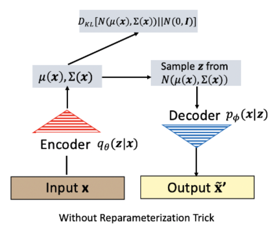
VAE: Encoder outputs distribution parameters, sample z from this distribution
The Reparameterization Trick
There's a problem: we can't backpropagate through a sampling operation. The reparameterization trick makes this differentiable:
Reparameterization Trick
Original: z ~ N(μ, σ²) — sampling breaks gradient flow
Reparameterized: z = μ + σ · ε, where ε ~ N(0, 1)
The randomness is now external (ε), and z is a deterministic function of μ, σ, and ε.
Gradients can flow through μ and σ back to the encoder!
def reparameterize(mu, log_var):
    """
    Reparameterization trick: z = mu + std * epsilon
    log_var used instead of var for numerical stability
    """
    std = torch.exp(0.5 * log_var)  # σ = exp(0.5 * log(σ²))
    eps = torch.randn_like(std)        # ε ~ N(0, 1)
    z = mu + std * eps                 # z = μ + σ * ε
    return z
VAE Loss Function
The VAE loss has two components that work together:
VAE Evidence Lower Bound (ELBO)
L = -𝔼q(z|x)[log p(x|z)] + KL(q(z|x) || p(z))
Reconstruction Loss: -𝔼[log p(x|z)] — how well can we reconstruct x from z?
KL Divergence: KL(q(z|x) || p(z)) — how close is our learned distribution to the prior?
Reconstruction loss forces the model to preserve information about x in z.
KL divergence regularizes the latent space, pushing it toward a standard normal distribution N(0, I). This ensures:
- The latent space is continuous — nearby points decode to similar outputs
- The latent space is complete — we can sample anywhere and get valid outputs
- We can generate new samples by sampling z ~ N(0, I) and decoding
Closed-Form KL Divergence
For Gaussian distributions, the KL divergence has a closed form:
KL Divergence for Gaussians
If q(z|x) = N(μ, σ²) and p(z) = N(0, 1):
KL(q||p) = -½ Σj (1 + log(σj²) - μj² - σj²)
This can be computed analytically — no sampling required!
def vae_loss(x, x_reconstructed, mu, log_var):
    """
    VAE loss = Reconstruction + KL divergence
    """
    # Reconstruction loss (binary cross-entropy for binary data)
    recon_loss = F.binary_cross_entropy(x_reconstructed, x, reduction='sum')

    # KL divergence: -0.5 * sum(1 + log(σ²) - μ² - σ²)
    kl_loss = -0.5 * torch.sum(1 + log_var - mu.pow(2) - log_var.exp())

    return recon_loss + kl_loss
Generation with VAEs
Once trained, generating new samples is simple:
# Generate new synthetic patient
def generate_samples(decoder, num_samples, latent_dim):
    # Sample from prior: z ~ N(0, I)
    z = torch.randn(num_samples, latent_dim)

    # Decode to data space
    with torch.no_grad():
        generated = decoder(z)

    return generated

# Generate 100 synthetic patients
synthetic_patients = generate_samples(vae.decoder, 100, latent_dim=64)
Latent Space Interpolation
A key advantage of VAEs: the latent space is smooth and meaningful. We can interpolate between patients:
# Interpolate between two patients
def interpolate(vae, x1, x2, steps=10):
    # Encode both patients
    mu1, _ = vae.encode(x1)
    mu2, _ = vae.encode(x2)

    # Linear interpolation in latent space
    interpolations = []
    for alpha in np.linspace(0, 1, steps):
        z = (1 - alpha) * mu1 + alpha * mu2
        x_interp = vae.decode(z)
        interpolations.append(x_interp)

    return interpolations

# Result: smooth transition from patient 1's conditions to patient 2's
VAE Application: Molecule Generation for Drug Discovery
One of the most exciting applications of generative models in healthcare is de novo drug design: generating novel molecular structures with desired therapeutic properties.
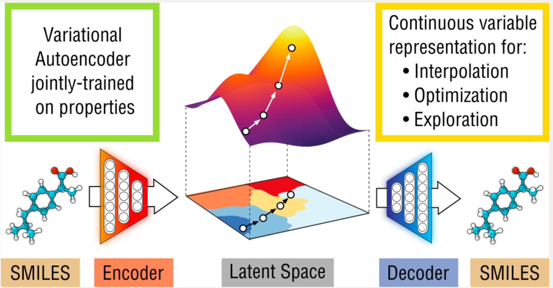
VAE for molecule generation: encode molecular structure, manipulate in latent space, decode to novel molecules
The Drug Discovery Problem
Traditional drug discovery is slow and expensive:
- Chemical space is vast: ~1060 possible drug-like molecules
- High-throughput screening tests ~106 compounds — a tiny fraction
- Average time to market: 10-15 years
- Average cost: $2.6 billion per approved drug
Generative models can guide exploration by learning what makes molecules drug-like and generating candidates with desired properties.
Molecular Representations
Molecules can be represented in several ways:
| Representation | Example (Aspirin) | Pros/Cons |
|---|---|---|
| SMILES | CC(=O)OC1=CC=CC=C1C(=O)O | String format, easy to process; not unique |
| Molecular Graph | Nodes=atoms, edges=bonds | Preserves structure; requires GNNs |
| Fingerprints | Binary vector of substructures | Fixed size; loses some information |
VAE for SMILES Strings
The simplest approach encodes SMILES strings character-by-character:
# Character-level VAE for molecules
class MoleculeVAE(nn.Module):
    def __init__(self, vocab_size, max_len, latent_dim, hidden_dim=256):
        super().__init__()

        # Encoder: SMILES → latent
        self.encoder = nn.GRU(vocab_size, hidden_dim, batch_first=True)
        self.fc_mu = nn.Linear(hidden_dim, latent_dim)
        self.fc_logvar = nn.Linear(hidden_dim, latent_dim)

        # Decoder: latent → SMILES
        self.fc_decode = nn.Linear(latent_dim, hidden_dim)
        self.decoder = nn.GRU(vocab_size, hidden_dim, batch_first=True)
        self.fc_out = nn.Linear(hidden_dim, vocab_size)

        self.max_len = max_len

    def encode(self, x):
        # x: one-hot encoded SMILES [batch, seq_len, vocab_size]
        _, h = self.encoder(x)
        h = h.squeeze(0)
        mu = self.fc_mu(h)
        logvar = self.fc_logvar(h)
        return mu, logvar

    def decode(self, z, max_len=None):
        # Autoregressive decoding
        max_len = max_len or self.max_len
        h = self.fc_decode(z).unsqueeze(0)

        # Start with start token
        outputs = []
        # ... autoregressive generation ...
        return outputs
Property Optimization in Latent Space
The real power: we can optimize molecular properties by moving in latent space:
🧬 Latent Space Drug Design
- Encode a known active molecule to z
- Train a property predictor on latent vectors (e.g., binding affinity)
- Gradient ascent in latent space toward desired properties
- Decode optimized z to novel molecular structure
This enables targeted generation of molecules with specific properties!
MolGAN: Graph-based Molecule Generation
MolGAN (De Cao & Kipf, 2018) generates molecular graphs directly using a GAN with graph neural networks:
- Generator: Outputs adjacency matrix and node features
- Discriminator: Graph neural network that processes molecular graphs
- Reward network: Predicts molecular properties (solubility, drug-likeness)
The reward network allows reinforcement learning to guide generation toward desired properties.
GAN vs VAE: When to Use Which?
Both GANs and VAEs can generate synthetic data, but they have different strengths:
| Aspect | GAN | VAE |
|---|---|---|
| Sample Quality | Sharper, more realistic | Slightly blurrier |
| Training Stability | Difficult, mode collapse risk | Stable, well-defined loss |
| Latent Space | Not explicitly regularized | Smooth, interpretable |
| Mode Coverage | May miss modes (mode collapse) | Better coverage of distribution |
| Likelihood | Cannot compute P(x) | Provides lower bound on P(x) |
| Interpolation | Not guaranteed to work | Smooth interpolation |
| Attribute Control | Conditional GAN needed | Natural via latent manipulation |
🏥 Recommendations for Healthcare
Use GANs when:
- Sample realism is critical (medical images)
- You have large training datasets
- You can invest in hyperparameter tuning
Use VAEs when:
- You need interpretable latent representations
- You want to interpolate between patients/molecules
- Training stability is important
- You need uncertainty estimates
Practical Implementation: VAE for Synthetic EHR
Let's build a complete VAE for generating synthetic patient records. We'll work with binary multi-hot encoded diagnoses — the same representation used in medical embeddings.
Data Format
Each patient is represented as a binary vector where 1 indicates presence of a diagnosis code:
# Patient representation
# Assume 1000 possible diagnosis codes
# Patient with diabetes (idx 250), hypertension (idx 401), CKD (idx 585):
# x = [0, 0, ..., 1, ..., 1, ..., 1, ..., 0]  # 1s at indices 250, 401, 585
#                  ^250    ^401    ^585
VAE Architecture
import torch
import torch.nn as nn
import torch.nn.functional as F
import numpy as np

class EHR_VAE(nn.Module):
    """
    Variational Autoencoder for binary EHR diagnosis codes.

    Input: Multi-hot encoded patient record [batch_size, num_codes]
    Output: Reconstructed record + latent parameters (mu, log_var)
    """

    def __init__(self, num_codes, hidden_dims=[512, 256], latent_dim=64):
        super().__init__()

        self.num_codes = num_codes
        self.latent_dim = latent_dim

        # ============ Encoder ============
        encoder_layers = []
        prev_dim = num_codes
        for hidden_dim in hidden_dims:
            encoder_layers.extend([
                nn.Linear(prev_dim, hidden_dim),
                nn.BatchNorm1d(hidden_dim),
                nn.ReLU(),
                nn.Dropout(0.2)
            ])
            prev_dim = hidden_dim

        self.encoder = nn.Sequential(*encoder_layers)

        # Latent space parameters
        self.fc_mu = nn.Linear(hidden_dims[-1], latent_dim)
        self.fc_logvar = nn.Linear(hidden_dims[-1], latent_dim)

        # ============ Decoder ============
        decoder_layers = []
        decoder_dims = [latent_dim] + hidden_dims[::-1]  # Reverse hidden dims

        for i in range(len(decoder_dims) - 1):
            decoder_layers.extend([
                nn.Linear(decoder_dims[i], decoder_dims[i+1]),
                nn.BatchNorm1d(decoder_dims[i+1]),
                nn.ReLU(),
                nn.Dropout(0.2)
            ])

        # Output layer
        decoder_layers.append(nn.Linear(decoder_dims[-1], num_codes))
        decoder_layers.append(nn.Sigmoid())  # Binary output

        self.decoder = nn.Sequential(*decoder_layers)

    def encode(self, x):
        """Encode input to latent distribution parameters."""
        h = self.encoder(x)
        mu = self.fc_mu(h)
        logvar = self.fc_logvar(h)
        return mu, logvar

    def reparameterize(self, mu, logvar):
        """Reparameterization trick: z = mu + std * epsilon"""
        std = torch.exp(0.5 * logvar)
        eps = torch.randn_like(std)
        return mu + std * eps

    def decode(self, z):
        """Decode latent vector to reconstructed input."""
        return self.decoder(z)

    def forward(self, x):
        """Full forward pass: encode, sample, decode."""
        mu, logvar = self.encode(x)
        z = self.reparameterize(mu, logvar)
        x_recon = self.decode(z)
        return x_recon, mu, logvar

    def generate(self, num_samples):
        """Generate new synthetic patients."""
        with torch.no_grad():
            # Sample from prior N(0, I)
            z = torch.randn(num_samples, self.latent_dim)
            samples = self.decode(z)
        return samples


# Initialize model
num_codes = 1000  # Vocabulary of diagnosis codes
vae = EHR_VAE(num_codes=num_codes, hidden_dims=[512, 256], latent_dim=64)
print(vae)
# Model architecture:
# EHR_VAE(
#   (encoder): Sequential(
#     (0): Linear(in_features=1000, out_features=512)
#     (1): BatchNorm1d(512)
#     (2): ReLU()
#     (3): Dropout(p=0.2)
#     (4): Linear(in_features=512, out_features=256)
#     (5): BatchNorm1d(256)
#     (6): ReLU()
#     (7): Dropout(p=0.2)
#   )
#   (fc_mu): Linear(in_features=256, out_features=64)
#   (fc_logvar): Linear(in_features=256, out_features=64)
#   (decoder): Sequential(...)
# )
Loss Function
def vae_loss_function(x_recon, x, mu, logvar, beta=1.0):
    """
    VAE loss = Reconstruction + β * KL divergence

    Args:
        x_recon: Reconstructed input [batch, num_codes]
        x: Original input [batch, num_codes]
        mu: Latent mean [batch, latent_dim]
        logvar: Latent log variance [batch, latent_dim]
        beta: Weight for KL term (β-VAE)

    Returns:
        total_loss, recon_loss, kl_loss
    """
    # Reconstruction loss: Binary Cross Entropy
    # Sum over codes, mean over batch
    recon_loss = F.binary_cross_entropy(x_recon, x, reduction='none')
    recon_loss = recon_loss.sum(dim=1).mean()

    # KL divergence: -0.5 * sum(1 + log(σ²) - μ² - σ²)
    kl_loss = -0.5 * torch.sum(1 + logvar - mu.pow(2) - logvar.exp(), dim=1)
    kl_loss = kl_loss.mean()

    # Total loss
    total_loss = recon_loss + beta * kl_loss

    return total_loss, recon_loss, kl_loss
Training Loop
from torch.utils.data import DataLoader, TensorDataset
import torch.optim as optim

def train_vae(vae, train_data, num_epochs=50, batch_size=64, lr=1e-3, beta=1.0):
    """
    Train VAE on binary EHR data.

    Args:
        vae: EHR_VAE model
        train_data: numpy array [num_patients, num_codes]
        num_epochs: Training epochs
        batch_size: Batch size
        lr: Learning rate
        beta: KL weight (use β < 1 for better reconstruction)
    """
    device = torch.device("cuda" if torch.cuda.is_available() else "cpu")
    vae = vae.to(device)

    # Create DataLoader
    dataset = TensorDataset(torch.tensor(train_data, dtype=torch.float32))
    dataloader = DataLoader(dataset, batch_size=batch_size, shuffle=True)

    optimizer = optim.Adam(vae.parameters(), lr=lr)

    history = {'total_loss': [], 'recon_loss': [], 'kl_loss': []}

    for epoch in range(num_epochs):
        vae.train()
        epoch_total, epoch_recon, epoch_kl = 0, 0, 0

        for batch in dataloader:
            x = batch[0].to(device)

            optimizer.zero_grad()

            # Forward pass
            x_recon, mu, logvar = vae(x)

            # Compute loss
            total_loss, recon_loss, kl_loss = vae_loss_function(
                x_recon, x, mu, logvar, beta=beta
            )

            # Backward pass
            total_loss.backward()
            optimizer.step()

            epoch_total += total_loss.item()
            epoch_recon += recon_loss.item()
            epoch_kl += kl_loss.item()

        # Record history
        n_batches = len(dataloader)
        history['total_loss'].append(epoch_total / n_batches)
        history['recon_loss'].append(epoch_recon / n_batches)
        history['kl_loss'].append(epoch_kl / n_batches)

        if (epoch + 1) % 10 == 0:
            print(f"Epoch {epoch+1:3d} | Total: {history['total_loss'][-1]:.2f} | "
                  f"Recon: {history['recon_loss'][-1]:.2f} | KL: {history['kl_loss'][-1]:.2f}")

    return history

# Train the model
# history = train_vae(vae, train_data, num_epochs=50, beta=0.5)
# Sample output:
# Epoch  10 | Total: 142.35 | Recon: 138.42 | KL: 7.86
# Epoch  20 | Total: 98.23 | Recon: 91.18 | KL: 14.10
# Epoch  30 | Total: 76.45 | Recon: 67.32 | KL: 18.26
# Epoch  40 | Total: 64.12 | Recon: 53.89 | KL: 20.46
# Epoch  50 | Total: 58.34 | Recon: 47.21 | KL: 22.26
Generating Synthetic Patients
def generate_synthetic_patients(vae, num_patients, threshold=0.5):
    """
    Generate synthetic patient records.

    Args:
        vae: Trained VAE model
        num_patients: Number of synthetic patients to generate
        threshold: Probability threshold for binary codes

    Returns:
        Binary array of synthetic patients [num_patients, num_codes]
    """
    vae.eval()

    with torch.no_grad():
        # Sample from prior
        z = torch.randn(num_patients, vae.latent_dim)

        # Decode to probabilities
        probs = vae.decode(z)

        # Threshold to binary
        synthetic = (probs > threshold).float().numpy()

    return synthetic

# Generate 1000 synthetic patients
# synthetic_patients = generate_synthetic_patients(vae, 1000)
# print(f"Generated {synthetic_patients.shape[0]} synthetic patients")
# print(f"Average codes per patient: {synthetic_patients.sum(axis=1).mean():.1f}")
Evaluating Synthetic Data Quality
def evaluate_synthetic_quality(real_data, synthetic_data):
    """
    Evaluate quality of synthetic data.

    Metrics:
    1. Dimension-wise probability difference
    2. Average codes per patient
    3. Code co-occurrence similarity
    """
    results = {}

    # 1. Dimension-wise probability (code prevalence)
    real_prevalence = real_data.mean(axis=0)
    synth_prevalence = synthetic_data.mean(axis=0)

    # Mean absolute difference
    prevalence_diff = np.abs(real_prevalence - synth_prevalence).mean()
    results['prevalence_MAE'] = prevalence_diff

    # Correlation of prevalences
    prevalence_corr = np.corrcoef(real_prevalence, synth_prevalence)[0, 1]
    results['prevalence_corr'] = prevalence_corr

    # 2. Average codes per patient
    real_avg_codes = real_data.sum(axis=1).mean()
    synth_avg_codes = synthetic_data.sum(axis=1).mean()
    results['real_avg_codes'] = real_avg_codes
    results['synth_avg_codes'] = synth_avg_codes

    # 3. Code co-occurrence (correlation matrix)
    # Select top 50 most common codes for efficiency
    top_codes = np.argsort(real_prevalence)[-50:]

    real_cooc = np.corrcoef(real_data[:, top_codes].T)
    synth_cooc = np.corrcoef(synthetic_data[:, top_codes].T)

    # Frobenius norm of difference
    cooc_diff = np.linalg.norm(real_cooc - synth_cooc, 'fro')
    results['cooccurrence_diff'] = cooc_diff

    return results

# Example evaluation output:
# {'prevalence_MAE': 0.0234,
#  'prevalence_corr': 0.9812,
#  'real_avg_codes': 8.3,
#  'synth_avg_codes': 7.9,
#  'cooccurrence_diff': 2.45}
Practical Implementation: Simple GAN for Tabular Medical Data
Now let's implement a basic GAN for generating tabular medical data. This is simpler than MedGAN but illustrates the core concepts.
Generator and Discriminator Networks
class Generator(nn.Module):
    """
    Generator network: transforms random noise into fake patient records.
    """
    def __init__(self, noise_dim, output_dim, hidden_dims=[256, 512, 256]):
        super().__init__()

        layers = []
        prev_dim = noise_dim

        for hidden_dim in hidden_dims:
            layers.extend([
                nn.Linear(prev_dim, hidden_dim),
                nn.BatchNorm1d(hidden_dim),
                nn.LeakyReLU(0.2),
            ])
            prev_dim = hidden_dim

        # Output layer with sigmoid for binary codes
        layers.append(nn.Linear(prev_dim, output_dim))
        layers.append(nn.Sigmoid())

        self.model = nn.Sequential(*layers)

    def forward(self, z):
        return self.model(z)


class Discriminator(nn.Module):
    """
    Discriminator network: classifies inputs as real or fake.
    """
    def __init__(self, input_dim, hidden_dims=[256, 128, 64]):
        super().__init__()

        layers = []
        prev_dim = input_dim

        for hidden_dim in hidden_dims:
            layers.extend([
                nn.Linear(prev_dim, hidden_dim),
                nn.LeakyReLU(0.2),
                nn.Dropout(0.3),
            ])
            prev_dim = hidden_dim

        # Output: probability that input is real
        layers.append(nn.Linear(prev_dim, 1))
        layers.append(nn.Sigmoid())

        self.model = nn.Sequential(*layers)

    def forward(self, x):
        return self.model(x)


# Initialize networks
noise_dim = 128
num_codes = 1000

generator = Generator(noise_dim=noise_dim, output_dim=num_codes)
discriminator = Discriminator(input_dim=num_codes)
GAN Training Loop
def train_gan(generator, discriminator, train_data, num_epochs=100,
              batch_size=64, noise_dim=128, lr_g=2e-4, lr_d=2e-4):
    """
    Train GAN on binary EHR data.

    Uses Binary Cross Entropy loss with alternating G/D updates.
    """
    device = torch.device("cuda" if torch.cuda.is_available() else "cpu")
    generator = generator.to(device)
    discriminator = discriminator.to(device)

    # Optimizers
    optimizer_G = optim.Adam(generator.parameters(), lr=lr_g, betas=(0.5, 0.999))
    optimizer_D = optim.Adam(discriminator.parameters(), lr=lr_d, betas=(0.5, 0.999))

    # Loss function
    criterion = nn.BCELoss()

    # Data loader
    dataset = TensorDataset(torch.tensor(train_data, dtype=torch.float32))
    dataloader = DataLoader(dataset, batch_size=batch_size, shuffle=True)

    history = {'d_loss': [], 'g_loss': [], 'd_real': [], 'd_fake': []}

    for epoch in range(num_epochs):
        epoch_d_loss, epoch_g_loss = 0, 0
        epoch_d_real, epoch_d_fake = 0, 0

        for batch in dataloader:
            real_data = batch[0].to(device)
            batch_size_actual = real_data.size(0)

            # Labels
            real_labels = torch.ones(batch_size_actual, 1).to(device)
            fake_labels = torch.zeros(batch_size_actual, 1).to(device)

            # ============ Train Discriminator ============
            optimizer_D.zero_grad()

            # Real data
            real_pred = discriminator(real_data)
            d_loss_real = criterion(real_pred, real_labels)

            # Fake data
            noise = torch.randn(batch_size_actual, noise_dim).to(device)
            fake_data = generator(noise).detach()
            fake_pred = discriminator(fake_data)
            d_loss_fake = criterion(fake_pred, fake_labels)

            # Combined discriminator loss
            d_loss = d_loss_real + d_loss_fake
            d_loss.backward()
            optimizer_D.step()

            # ============ Train Generator ============
            optimizer_G.zero_grad()

            noise = torch.randn(batch_size_actual, noise_dim).to(device)
            fake_data = generator(noise)
            fake_pred = discriminator(fake_data)

            # Generator wants discriminator to think fake is real
            g_loss = criterion(fake_pred, real_labels)
            g_loss.backward()
            optimizer_G.step()

            # Track metrics
            epoch_d_loss += d_loss.item()
            epoch_g_loss += g_loss.item()
            epoch_d_real += real_pred.mean().item()
            epoch_d_fake += fake_pred.mean().item()

        # Record history
        n_batches = len(dataloader)
        history['d_loss'].append(epoch_d_loss / n_batches)
        history['g_loss'].append(epoch_g_loss / n_batches)
        history['d_real'].append(epoch_d_real / n_batches)
        history['d_fake'].append(epoch_d_fake / n_batches)

        if (epoch + 1) % 20 == 0:
            print(f"Epoch {epoch+1:3d} | D_loss: {history['d_loss'][-1]:.3f} | "
                  f"G_loss: {history['g_loss'][-1]:.3f} | "
                  f"D(real): {history['d_real'][-1]:.3f} | "
                  f"D(fake): {history['d_fake'][-1]:.3f}")

    return history

# Train GAN
# history = train_gan(generator, discriminator, train_data, num_epochs=100)
# Sample output:
# Epoch  20 | D_loss: 1.245 | G_loss: 0.823 | D(real): 0.712 | D(fake): 0.341
# Epoch  40 | D_loss: 1.189 | G_loss: 0.891 | D(real): 0.683 | D(fake): 0.398
# Epoch  60 | D_loss: 1.156 | G_loss: 0.934 | D(real): 0.654 | D(fake): 0.421
# Epoch  80 | D_loss: 1.134 | G_loss: 0.967 | D(real): 0.632 | D(fake): 0.445
# Epoch 100 | D_loss: 1.112 | G_loss: 0.989 | D(real): 0.612 | D(fake): 0.468
Generating Samples from GAN
def generate_from_gan(generator, num_samples, noise_dim, threshold=0.5):
    """Generate synthetic patients using trained generator."""
    generator.eval()

    with torch.no_grad():
        noise = torch.randn(num_samples, noise_dim)
        probs = generator(noise)
        synthetic = (probs > threshold).float().numpy()

    return synthetic

# Generate and compare distributions
# synthetic_gan = generate_from_gan(generator, 1000, noise_dim)
# quality_metrics = evaluate_synthetic_quality(real_data, synthetic_gan)
Summary
We covered the theory and implementation of generative models for healthcare:
| Model | Key Idea | Strengths | Healthcare Applications |
|---|---|---|---|
| GAN | Adversarial training: Generator vs Discriminator | Sharp, realistic samples | Medical imaging, synthetic EHR |
| MedGAN | Autoencoder + GAN for discrete codes | Handles binary multi-label data | Privacy-preserving EHR generation |
| VAE | Probabilistic encoder, regularized latent space | Stable training, interpretable latent space | Patient representation, interpolation |
| MolVAE/MolGAN | Generate molecular structures | Property optimization in latent space | Drug discovery, lead optimization |
⚠️ Important Considerations for Healthcare
- Privacy validation: Synthetic data should be rigorously tested to ensure no real patient can be identified. Use differential privacy or membership inference attacks to validate.
- Distribution shift: Synthetic data may not capture rare but important patterns (outliers, rare diseases). Always validate with domain experts.
- Downstream utility: The true test is whether models trained on synthetic data perform well on real data tasks.
- Regulatory considerations: Even synthetic data may fall under regulations if derived from real patient data. Consult legal/compliance teams.
References
- Goodfellow et al. (2014). "Generative Adversarial Nets" — Original GAN paper, NIPS 2014
- Kingma & Welling (2014). "Auto-Encoding Variational Bayes" — VAE paper
- Choi et al. (2017). "Generating Multi-label Discrete Patient Records using Generative Adversarial Networks" — MedGAN
- De Cao & Kipf (2018). "MolGAN: An implicit generative model for small molecular graphs"
- Gómez-Bombarelli et al. (2018). "Automatic Chemical Design Using a Data-Driven Continuous Representation of Molecules" — Molecular VAE
- Yale et al. (2020). "Privacy Preserving Synthetic Health Data" — Survey on synthetic EHR generation