Medical Embeddings and Deep Neural Networks
"In healthcare data, similar conditions should live in similar neighborhoods."
August 2026 · Giacomo Saccaggi
The Representation Problem in Healthcare
Electronic Health Records (EHRs) contain rich information about patients: diagnosis codes (ICD-9/10), procedure codes (CPT), medications (NDC), lab results, and clinical notes. But how do we feed this heterogeneous data into machine learning models?
The naive approach is one-hot encoding: create a binary vector where each position corresponds to a possible diagnosis code. If a patient has diabetes (ICD-9: 250.00), we set that position to 1.
One-hot encoding treats all medical codes as equally distant from each other
The problem? With ~15,000 ICD-9 codes and ~70,000 ICD-10 codes, we get extremely sparse, high-dimensional vectors where:
- All codes are equidistant — "Type 2 Diabetes" is as far from "Type 1 Diabetes" as it is from "Fractured Tibia"
- No semantic relationships — the model can't learn that hypertension and heart disease are related
- Curse of dimensionality — most entries are zeros, making learning inefficient
What we need is a way to represent medical concepts as dense, low-dimensional vectors where similar conditions cluster together. This is where embeddings come in.
Word2Vec: Learning Distributed Representations
The breakthrough came from NLP. In 2013, Mikolov et al. introduced Word2Vec, a neural network that learns vector representations of words from their context. The key insight: "You shall know a word by the company it keeps."
The Skip-gram Model
Given a target word, predict the surrounding context words. If we see "patient was diagnosed with diabetes and prescribed metformin", the model learns that "diabetes" often appears near "diagnosed", "prescribed", and "metformin".
Skip-gram Objective
Maximize the probability of context words given the target word:
J(θ) = Σ(t,c)∈D log p(c|t)
Where the probability is computed using softmax:
p(c|t) = exp(vcT · vt) / Σw∈V exp(vwT · vt)
vt = embedding of target word, vc = embedding of context word, V = vocabulary
Skip-gram: predict context words from the center word
The Computational Problem
The softmax denominator requires summing over the entire vocabulary for every training example. With 15,000+ medical codes, this is prohibitively expensive.
Negative Sampling
Instead of computing the full softmax, we reformulate the problem as binary classification: distinguish real (target, context) pairs from fake ones.
Negative Sampling Objective
For each positive pair (t, c), sample k negative pairs (t, n) where n is a random word:
J(θ) = log σ(vcT · vt) + Σi=1k 𝔼n~P(w)[log σ(-vnT · vt)]
Where σ is the sigmoid function and P(w) is a noise distribution (typically unigram3/4)
This reduces complexity from O(|V|) to O(k) per example, where k is typically 5-20.
From Words to Medical Codes
The same principle applies to healthcare. Instead of words in sentences, we have medical codes in patient records. A patient's visit becomes a "sentence" of diagnosis codes, procedures, and medications.

Medical codes can be embedded using the same Word2Vec principles
Training Medical Embeddings
Given a corpus of patient records, we treat each visit as a context window:
# Patient visit: [Diabetes, Hypertension, Metformin, Lisinopril]
# Generate skip-gram pairs:
# (Diabetes, Hypertension), (Diabetes, Metformin), (Diabetes, Lisinopril)
# (Hypertension, Diabetes), (Hypertension, Metformin), ...

from gensim.models import Word2Vec

# Each patient's visits as a list of medical codes
patient_records = [
    ["250.00", "401.9", "metformin", "lisinopril"],  # Patient 1, Visit 1
    ["250.00", "272.4", "atorvastatin"],              # Patient 1, Visit 2
    ["414.01", "401.9", "aspirin", "metoprolol"],    # Patient 2, Visit 1
    # ... millions more visits
]

# Train Word2Vec on medical codes
model = Word2Vec(
    sentences=patient_records,
    vector_size=128,      # Embedding dimension
    window=5,              # Context window size
    min_count=5,           # Ignore rare codes
    sg=1,                  # Skip-gram (vs CBOW)
    negative=10,           # Negative samples per positive
    workers=4
)

# Get embedding for diabetes
diabetes_embedding = model.wv["250.00"]  # Shape: (128,)
Similarity Search: The Magic of Embeddings
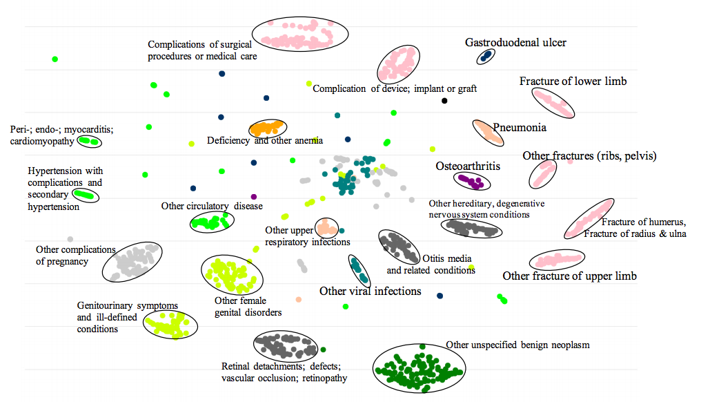
Once trained, embeddings capture semantic relationships. Similar diagnoses cluster together in the vector space:
Similar conditions cluster together in embedding space
# Find codes most similar to "Acute upper respiratory infection"
model.wv.most_similar("465.9", topn=5)

# Results:
# [("466.0", 0.89),   # Acute bronchitis
#  ("786.2", 0.85),   # Cough
#  ("461.9", 0.83),   # Acute sinusitis
#  ("462",   0.81),   # Acute pharyngitis
#  ("460",   0.79)]   # Common cold
Algebraic Operations on Medical Concepts
Perhaps the most remarkable property: embeddings support analogical reasoning. Just as "King - Man + Woman ≈ Queen" in word embeddings, medical embeddings exhibit similar behavior:
🧮 Medical Analogies
Hypertension + Obesity ≈ ?
Results: Type 2 Diabetes, Hyperlipidemia, Coronary Atherosclerosis
The model learned that hypertension combined with obesity risk factors leads to metabolic syndrome conditions!
# Hypertension + Obesity → what conditions?
result = model.wv.most_similar(
    positive=["401.9", "278.00"],  # Hypertension + Obesity
    topn=5
)
# [("250.00", 0.82),   # Type 2 Diabetes
#  ("272.4",  0.79),   # Hyperlipidemia
#  ("414.01", 0.76),   # Coronary atherosclerosis
#  ("427.31", 0.71),   # Atrial fibrillation
#  ("585.9",  0.68)]   # Chronic kidney disease
Patient Representation
Now that we have embeddings for individual medical codes, how do we represent an entire patient?
The simplest approach: sum (or average) the embeddings of all codes in the patient's history:
Patient Embedding
vpatient = Σc ∈ codes(patient) vc
Or with averaging: vpatient = (1/|codes|) × Σc vc
import numpy as np

def patient_embedding(patient_codes, model, aggregate='sum'):
    """Convert list of medical codes to patient vector."""
    embeddings = []
    for code in patient_codes:
        if code in model.wv:
            embeddings.append(model.wv[code])

    if not embeddings:
        return np.zeros(model.vector_size)

    embeddings = np.array(embeddings)
    if aggregate == 'sum':
        return embeddings.sum(axis=0)
    elif aggregate == 'mean':
        return embeddings.mean(axis=0)

# Patient with diabetes, hypertension, and CKD
patient_codes = ["250.00", "401.9", "585.9"]
patient_vec = patient_embedding(patient_codes, model)
print(patient_vec.shape)  # (128,)
This patient vector can now be used as input to any downstream model: mortality prediction, readmission risk, disease progression, etc.
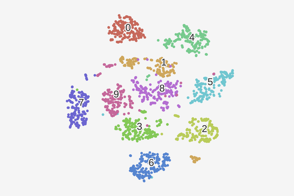
Visualizing Embeddings with t-SNE
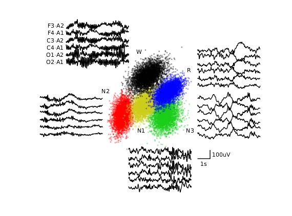
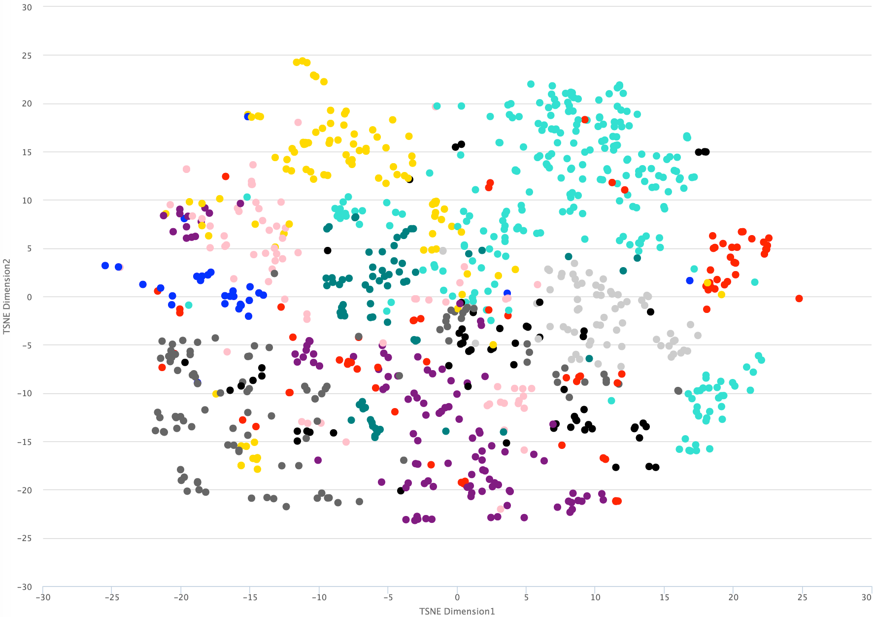
How do we visualize 128-dimensional embeddings? t-SNE (t-distributed Stochastic Neighbor Embedding) projects high-dimensional data to 2D while preserving local structure.

t-SNE projects high-dimensional embeddings to 2D for visualization
How t-SNE Works
t-SNE Algorithm
Step 1: Compute pairwise similarities in high-dimensional space using Gaussian kernel:
pj|i = exp(-||xi - xj||² / 2σi²) / Σk≠i exp(-||xi - xk||² / 2σi²)
Step 2: Compute similarities in low-dimensional space using Student t-distribution (heavier tails):
qij = (1 + ||yi - yj||²)-1 / Σk≠l (1 + ||yk - yl||²)-1
Step 3: Minimize KL divergence between P and Q:
KL(P||Q) = Σi Σj pij log(pij / qij)
The Student t-distribution is crucial: its heavy tails allow dissimilar points to be pushed far apart in the low-dimensional space, preventing the "crowding problem" where everything collapses to the center.
from sklearn.manifold import TSNE
import matplotlib.pyplot as plt

# Get embeddings for all medical codes
codes = list(model.wv.key_to_index.keys())
embeddings = np.array([model.wv[c] for c in codes])

# Apply t-SNE
tsne = TSNE(n_components=2, perplexity=30, random_state=42)
embeddings_2d = tsne.fit_transform(embeddings)

# Visualize
plt.figure(figsize=(12, 8))
plt.scatter(embeddings_2d[:, 0], embeddings_2d[:, 1], alpha=0.5, s=10)
plt.title("Medical Code Embeddings (t-SNE)")
plt.show()
Beyond Word2Vec: Med2Vec
Standard Word2Vec treats medical codes as independent tokens. But healthcare data has additional structure:
- Visit-level co-occurrence: codes appearing in the same visit are related
- Sequential structure: the order of visits matters (disease progression)
- Demographics: patient age, gender affect disease patterns
Med2Vec extends Word2Vec with a multi-layer architecture that captures both code-level and visit-level representations.
Med2Vec learns both code embeddings and visit embeddings
Med2Vec Architecture
| Layer | Input | Output | Purpose |
|---|---|---|---|
| Code Embedding | One-hot code | Dense vector | Learn code representations |
| Visit Embedding | Sum of code embeddings | Visit vector | Aggregate codes in a visit |
| Softmax (codes) | Visit embedding | Code probabilities | Predict codes in current visit |
| Softmax (visits) | Visit embedding | Next visit codes | Predict codes in adjacent visits |
The key innovation: Med2Vec jointly optimizes for within-visit co-occurrence and between-visit sequences:
Med2Vec Objective
L = Lcode + Lvisit
Lcode: predict codes from visit embedding (within-visit structure)
Lvisit: predict next visit's codes from current visit embedding (sequential structure)
MiME: Multilevel Medical Embedding
Real healthcare data is even more structured. A visit contains not just diagnoses, but also the treatments prescribed for each diagnosis. MiME captures this hierarchical structure.
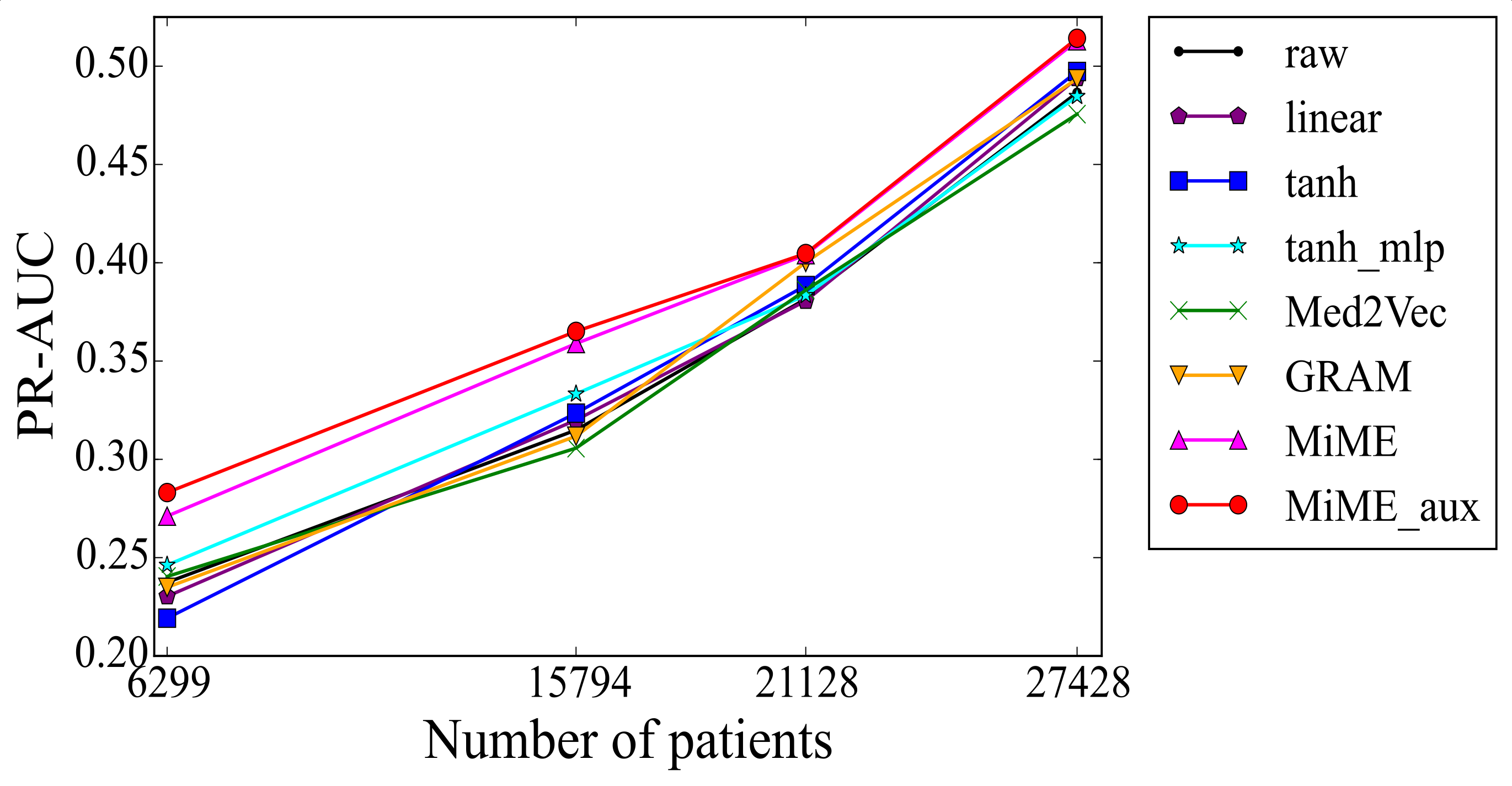
MiME captures diagnosis-treatment relationships within visits
MiME's Hierarchical Structure
- Treatment embedding: procedures/medications get their own vectors
- Diagnosis embedding: conditioned on associated treatments
- Visit embedding: aggregation of diagnosis-treatment pairs
- Patient embedding: sequence of visit embeddings
Auxiliary Prediction Tasks
MiME adds auxiliary tasks during training to learn richer representations:
- Diagnosis → Treatment: given a diagnosis, predict likely treatments
- Treatment → Diagnosis: given treatments, predict diagnoses
- Visit → Next Visit: predict future diagnoses from current visit
These auxiliary tasks force the model to learn semantically meaningful relationships, not just co-occurrence statistics.
Practical Implementation: DNN for Mortality Prediction
Let's build a complete deep neural network for predicting in-hospital mortality using PyTorch. We'll work with MIMIC-III style EHR data.
Data Format
Our dataset contains patient visits with diagnosis codes and a binary mortality label:
# Sample data structure
# patient_id | visit_diagnoses                    | mortality
# 1          | [250.00, 401.9, 585.9]             | 0
# 2          | [414.01, 427.31, 428.0, 518.81]    | 1
# 3          | [496, 786.05, 491.21]              | 0
Multi-hot Encoding
Each patient's diagnoses are encoded as a multi-hot vector (multiple 1s, unlike one-hot):
import numpy as np
import torch
from torch.utils.data import Dataset, DataLoader

class EHRDataset(Dataset):
    """Dataset for EHR diagnosis codes."""

    def __init__(self, diagnoses_list, labels, num_codes):
        """
        Args:
            diagnoses_list: List of lists, each inner list contains code indices
            labels: Binary mortality labels
            num_codes: Total number of unique diagnosis codes
        """
        self.diagnoses_list = diagnoses_list
        self.labels = labels
        self.num_codes = num_codes

    def __len__(self):
        return len(self.labels)

    def __getitem__(self, idx):
        # Create multi-hot vector
        multi_hot = np.zeros(self.num_codes, dtype=np.float32)
        for code_idx in self.diagnoses_list[idx]:
            multi_hot[code_idx] = 1.0

        return (
            torch.tensor(multi_hot),
            torch.tensor(self.labels[idx], dtype=torch.long)
        )

# Example usage
num_codes = 1000  # Vocabulary size
train_diagnoses = [[10, 50, 200], [5, 100, 300, 450], ...]
train_labels = [0, 1, ...]

dataset = EHRDataset(train_diagnoses, train_labels, num_codes)
dataloader = DataLoader(dataset, batch_size=32, shuffle=True)
DNN Architecture
A feedforward neural network with fully connected layers, ReLU activations, and dropout for regularization:
import torch.nn as nn
import torch.nn.functional as F

class MortalityDNN(nn.Module):
    """Deep Neural Network for mortality prediction."""

    def __init__(self, input_dim, hidden_dims=[512, 256, 128], dropout=0.3):
        """
        Args:
            input_dim: Number of diagnosis codes (vocabulary size)
            hidden_dims: List of hidden layer dimensions
            dropout: Dropout probability
        """
        super().__init__()

        layers = []
        prev_dim = input_dim

        for hidden_dim in hidden_dims:
            layers.extend([
                nn.Linear(prev_dim, hidden_dim),
                nn.ReLU(),
                nn.Dropout(dropout)
            ])
            prev_dim = hidden_dim

        self.hidden_layers = nn.Sequential(*layers)
        self.output_layer = nn.Linear(prev_dim, 2)  # Binary classification

    def forward(self, x):
        """
        Args:
            x: Multi-hot encoded diagnoses [batch_size, num_codes]
        Returns:
            logits: [batch_size, 2]
        """
        h = self.hidden_layers(x)
        logits = self.output_layer(h)
        return logits

# Initialize model
model = MortalityDNN(
    input_dim=1000,
    hidden_dims=[512, 256, 128],
    dropout=0.3
)
print(model)
# Model architecture output:
# MortalityDNN(
#   (hidden_layers): Sequential(
#     (0): Linear(in_features=1000, out_features=512)
#     (1): ReLU()
#     (2): Dropout(p=0.3)
#     (3): Linear(in_features=512, out_features=256)
#     (4): ReLU()
#     (5): Dropout(p=0.3)
#     (6): Linear(in_features=256, out_features=128)
#     (7): ReLU()
#     (8): Dropout(p=0.3)
#   )
#   (output_layer): Linear(in_features=128, out_features=2)
# )
Training Loop
import torch.optim as optim
from sklearn.metrics import roc_auc_score

def train_epoch(model, dataloader, criterion, optimizer, device):
    """Train for one epoch."""
    model.train()
    total_loss = 0

    for batch_x, batch_y in dataloader:
        batch_x = batch_x.to(device)
        batch_y = batch_y.to(device)

        optimizer.zero_grad()
        logits = model(batch_x)
        loss = criterion(logits, batch_y)
        loss.backward()
        optimizer.step()

        total_loss += loss.item()

    return total_loss / len(dataloader)


def evaluate(model, dataloader, device):
    """Evaluate model and return AUROC."""
    model.eval()
    all_probs = []
    all_labels = []

    with torch.no_grad():
        for batch_x, batch_y in dataloader:
            batch_x = batch_x.to(device)
            logits = model(batch_x)
            probs = F.softmax(logits, dim=1)[:, 1]  # P(mortality=1)

            all_probs.extend(probs.cpu().numpy())
            all_labels.extend(batch_y.numpy())

    auroc = roc_auc_score(all_labels, all_probs)
    return auroc


# Training setup
device = torch.device("cuda" if torch.cuda.is_available() else "cpu")
model = model.to(device)

criterion = nn.CrossEntropyLoss()
optimizer = optim.Adam(model.parameters(), lr=0.001)

# Training loop
num_epochs = 20
for epoch in range(num_epochs):
    train_loss = train_epoch(model, train_loader, criterion, optimizer, device)
    val_auroc = evaluate(model, val_loader, device)

    print(f"Epoch {epoch+1:2d} | Loss: {train_loss:.4f} | Val AUROC: {val_auroc:.4f}")
# Sample output:
# Epoch  1 | Loss: 0.6821 | Val AUROC: 0.6234
# Epoch  2 | Loss: 0.5943 | Val AUROC: 0.7012
# Epoch  3 | Loss: 0.5234 | Val AUROC: 0.7456
# ...
# Epoch 20 | Loss: 0.3012 | Val AUROC: 0.8234
DNN with Pre-trained Embeddings
Instead of learning from scratch with multi-hot inputs, we can use pre-trained medical embeddings:
class EmbeddingDNN(nn.Module):
    """DNN with pre-trained medical code embeddings."""

    def __init__(self, embedding_matrix, hidden_dims=[256, 128], dropout=0.3, freeze_embeddings=True):
        """
        Args:
            embedding_matrix: Pre-trained embeddings [num_codes, embed_dim]
            hidden_dims: Hidden layer dimensions
            dropout: Dropout probability
            freeze_embeddings: If True, don't update embeddings during training
        """
        super().__init__()

        num_codes, embed_dim = embedding_matrix.shape

        # Embedding layer initialized with pre-trained weights
        self.embedding = nn.Embedding(num_codes, embed_dim)
        self.embedding.weight.data.copy_(torch.tensor(embedding_matrix))

        if freeze_embeddings:
            self.embedding.weight.requires_grad = False

        # Hidden layers
        layers = []
        prev_dim = embed_dim
        for hidden_dim in hidden_dims:
            layers.extend([
                nn.Linear(prev_dim, hidden_dim),
                nn.ReLU(),
                nn.Dropout(dropout)
            ])
            prev_dim = hidden_dim

        self.hidden_layers = nn.Sequential(*layers)
        self.output_layer = nn.Linear(prev_dim, 2)

    def forward(self, code_indices, code_mask):
        """
        Args:
            code_indices: [batch_size, max_codes] - padded code indices
            code_mask: [batch_size, max_codes] - 1 for real codes, 0 for padding
        Returns:
            logits: [batch_size, 2]
        """
        # Get embeddings: [batch_size, max_codes, embed_dim]
        embeds = self.embedding(code_indices)

        # Masked average pooling
        mask_expanded = code_mask.unsqueeze(-1).float()  # [batch, max_codes, 1]
        embeds_masked = embeds * mask_expanded
        sum_embeds = embeds_masked.sum(dim=1)  # [batch, embed_dim]
        count = mask_expanded.sum(dim=1).clamp(min=1)  # Avoid division by zero
        patient_embed = sum_embeds / count  # [batch, embed_dim]

        # Forward through hidden layers
        h = self.hidden_layers(patient_embed)
        logits = self.output_layer(h)
        return logits

# Load pre-trained Word2Vec embeddings
embedding_matrix = np.array([model.wv[code] for code in code_vocabulary])

embed_model = EmbeddingDNN(
    embedding_matrix=embedding_matrix,
    hidden_dims=[256, 128],
    freeze_embeddings=True
)
💡 Embedding vs Multi-hot
Multi-hot input: Model learns representations from scratch. Requires more data and compute.
Pre-trained embeddings: Leverage knowledge from large corpora. Better generalization with limited labeled data.
In practice, pre-trained embeddings often improve AUROC by 2-5% on small datasets.
Complete Training Pipeline
Putting it all together — a complete, runnable example:
import numpy as np
import torch
import torch.nn as nn
import torch.optim as optim
from torch.utils.data import Dataset, DataLoader
from sklearn.metrics import roc_auc_score
from sklearn.model_selection import train_test_split

# ============ Data Preparation ============
def load_ehr_data(filepath):
    """Load EHR data from file.

    Expected format: each line is "code1,code2,...|label"
    """
    diagnoses = []
    labels = []

    with open(filepath, 'r') as f:
        for line in f:
            codes_str, label = line.strip().split('|')
            codes = codes_str.split(',')
            diagnoses.append(codes)
            labels.append(int(label))

    return diagnoses, labels


def build_vocabulary(diagnoses_list):
    """Build code-to-index mapping."""
    all_codes = set()
    for codes in diagnoses_list:
        all_codes.update(codes)

    code_to_idx = {code: idx for idx, code in enumerate(sorted(all_codes))}
    return code_to_idx


def encode_diagnoses(diagnoses_list, code_to_idx):
    """Convert code strings to indices."""
    encoded = []
    for codes in diagnoses_list:
        encoded.append([code_to_idx[c] for c in codes if c in code_to_idx])
    return encoded


# ============ Model Training ============
def train_model(model, train_loader, val_loader, num_epochs=20, lr=0.001):
    """Full training loop with early stopping."""
    device = torch.device("cuda" if torch.cuda.is_available() else "cpu")
    model = model.to(device)

    criterion = nn.CrossEntropyLoss()
    optimizer = optim.Adam(model.parameters(), lr=lr)

    best_auroc = 0
    patience = 5
    patience_counter = 0

    for epoch in range(num_epochs):
        # Training
        model.train()
        total_loss = 0
        for batch_x, batch_y in train_loader:
            batch_x, batch_y = batch_x.to(device), batch_y.to(device)

            optimizer.zero_grad()
            logits = model(batch_x)
            loss = criterion(logits, batch_y)
            loss.backward()
            optimizer.step()
            total_loss += loss.item()

        # Validation
        model.eval()
        all_probs, all_labels = [], []
        with torch.no_grad():
            for batch_x, batch_y in val_loader:
                batch_x = batch_x.to(device)
                probs = torch.softmax(model(batch_x), dim=1)[:, 1]
                all_probs.extend(probs.cpu().numpy())
                all_labels.extend(batch_y.numpy())

        val_auroc = roc_auc_score(all_labels, all_probs)
        avg_loss = total_loss / len(train_loader)

        print(f"Epoch {epoch+1:2d} | Loss: {avg_loss:.4f} | Val AUROC: {val_auroc:.4f}")

        # Early stopping
        if val_auroc > best_auroc:
            best_auroc = val_auroc
            patience_counter = 0
            torch.save(model.state_dict(), "best_model.pt")
        else:
            patience_counter += 1
            if patience_counter >= patience:
                print(f"Early stopping at epoch {epoch+1}")
                break

    return best_auroc
Results Comparison
Typical results on MIMIC-III mortality prediction:
| Method | Input Type | Val AUROC | Test AUROC |
|---|---|---|---|
| Logistic Regression | Multi-hot | 0.782 | 0.775 |
| Random Forest | Multi-hot | 0.801 | 0.789 |
| DNN (3 layers) | Multi-hot | 0.823 | 0.812 |
| DNN + Word2Vec | Embeddings | 0.841 | 0.834 |
| DNN + Med2Vec | Embeddings | 0.856 | 0.849 |
Key observations:
- DNNs outperform classical ML methods on this task
- Pre-trained embeddings provide consistent improvements
- Med2Vec > Word2Vec due to capturing visit-level structure
Summary
We covered the theory and practice of medical embeddings:
| Concept | Key Idea | Use Case |
|---|---|---|
| Word2Vec | Learn code vectors from co-occurrence | Basic code embeddings |
| Negative Sampling | Efficient training via binary classification | Scale to large vocabularies |
| Patient Embedding | Sum/average of code embeddings | Input to downstream models |
| t-SNE | Visualize high-dim embeddings in 2D | Exploratory analysis |
| Med2Vec | Visit-level + sequential structure | Richer patient representations |
| MiME | Diagnosis-treatment hierarchies | Treatment recommendation |
| DNN | Multi-layer feedforward network | Mortality/readmission prediction |
⚠️ Important Considerations
- Data quality: EHR data is messy — missing codes, coding errors, temporal shifts
- Class imbalance: Mortality is rare (~3-5%). Use class weights or oversampling
- Temporal validity: Train on past, test on future. Never leak future information
- Interpretability: Clinicians need to understand predictions. Consider attention mechanisms
References
- Mikolov et al. (2013). "Efficient Estimation of Word Representations in Vector Space" — Original Word2Vec paper
- Choi et al. (2016). "Multi-layer Representation Learning for Medical Concepts" — Med2Vec
- Choi et al. (2017). "MiME: Multilevel Medical Embedding" — MiME architecture
- van der Maaten & Hinton (2008). "Visualizing Data using t-SNE"
- Johnson et al. (2016). "MIMIC-III, a freely accessible critical care database"